Softmax Activation Function: Everything You Need to Know | Pinecone

Softmax Activation

Have you ever trained a neural network to solve the problem of multiclass classification? If yes, you know that the raw outputs of the neural network are often very difficult to interpret. The softmax activation function simplifies this for you by making the neural network’s outputs easier to interpret!

The softmax activation function transforms the raw outputs of the neural network into a vector of probabilities, essentially a probability distribution over the input classes. Consider a multiclass classification problem with N classes. The softmax activation returns an output vector that is N entries long, with the entry at index i corresponding to the probability of a particular input belonging to the class i.

In this tutorial, you’ll learn all about the softmax activation function. You’ll start by reviewing the basics of multiclass classification, then proceed to understand why you cannot use the sigmoid or argmax activations in the output layer for multiclass classification problems.

Finally, you’ll learn the mathematical formulation of the softmax function and implement it in Python.

Let’s get started.

Mục Lục

Multiclass Classification Revisited

Recall that in binary classification, there are only two possible classes. For example, a ConvNet trained to classify whether or not a given image is a panda is a binary classifier, whereas, in multiclass classification, there are more than two possible classes.

Let’s consider the following example: You’re given a dataset containing images of pandas, seals, and ducks. You’d like to train a neural network to predict whether a previously unseen image is that of a seal, a panda, or a duck.

Notice how the input class labels below are one-hot encoded, and the classes are mutually exclusive. In this context, mutual exclusivity means that a given image can only be one of {seal, panda, duck} at a time.

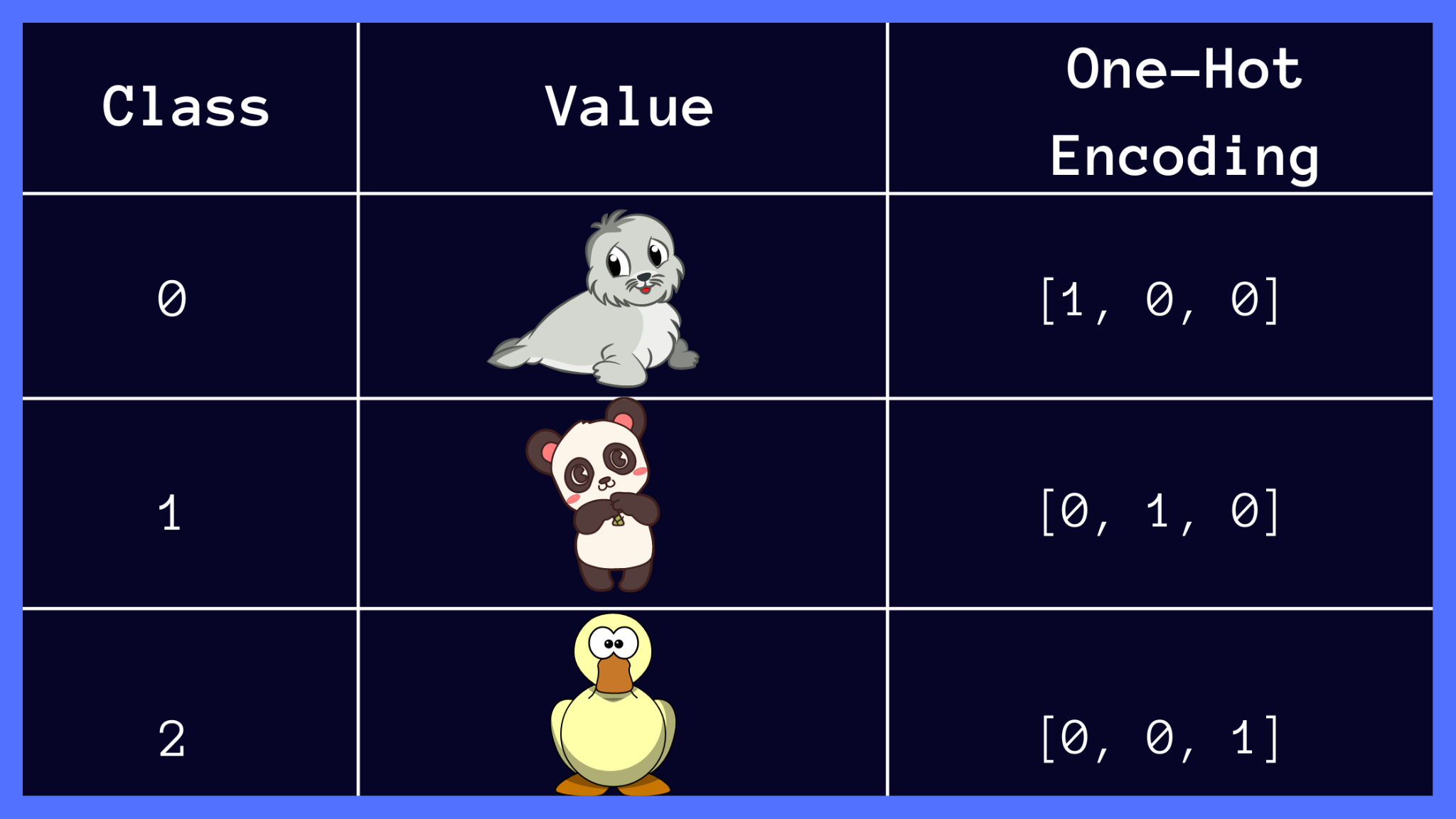
Multiclass Classification Example (Image by the author)

Can You Use Sigmoid or Argmax Activations Instead?

In this section, you’ll learn why the sigmoid and argmax functions are not the optimal choices for the output layer in a multiclass classification problem.

Limitations of the Sigmoid Function

Mathematically, the sigmoid activation function is given by the following equation, and it squishes all inputs onto the range [0, 1].

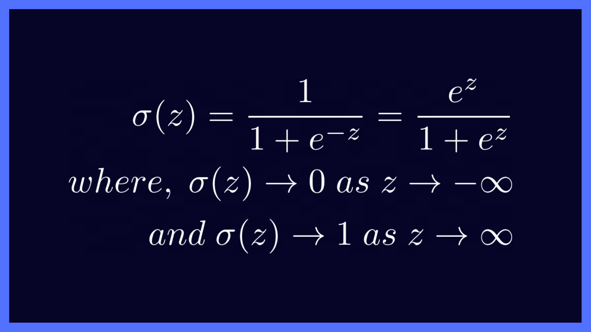
Sigmoid Function Equation (Image by the author)

The sigmoid function takes in any real number as the input and maps it to a number between 0 and 1. This is exactly why it’s well-suited for binary classification.

▶️ You may run the following code cell to plot the values of the sigmoid function over a range of numbers.

import
 numpy as np
import
 seaborn as sns

def
 sigmoid(x):
  exp_x =
 np.exp(x)
  return
 np.
divide(exp_x,(1
 + exp_x))
  
x =
 np.
linspace(-
10
,10
,num=
200)
exp_x =
 np.exp(x)
sigmoid_arr = sigmoid(x)

sns.set_theme()
sns.
lineplot(x =
 x,y =
 sigmoid_arr).
set(title=
'Sigmoid Function')

Sigmoid Function Plot
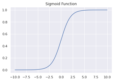
Plot of the Sigmoid Function

Let’s go back to our example of classifying whether an input image is that of a panda or not. In this case, let z be the raw output of the neural network. If σ(z) is the probability that the given image belongs to class 1 (is a panda), then 1 – σ(z) is the probability that the given image does not belong to class 1 and is not a panda. You can think of σ(z) as a probability score.

You can now fix a threshold, say T, and predict that class whose probability score is greater than the chosen threshold.

However, this won’t quite work when you have more than two classes. Softmax to the rescue!

In fact, you can think of the softmax function as a vector generalization of the sigmoid activation. We’ll revisit this later to confirm that for binary classification—when N = 2—the softmax and sigmoid activations are equivalent.

Limitations of the Argmax Function

The argmax function returns the index of the maximum value in the input array.

Let’s suppose the neural network’s raw output vector is given by z = [0.25, 1.23, -0.8]. In this case, the maximum value is 1.23 and it occurs at index 1. In our image classification example, index 1 corresponds to the second class—and the image is predicted to be that of a panda.

In vector notation, you’ll have 1 at the index where the maximum occurs (at index 1 for the vector z). And you’ll have 0 at all other indices.

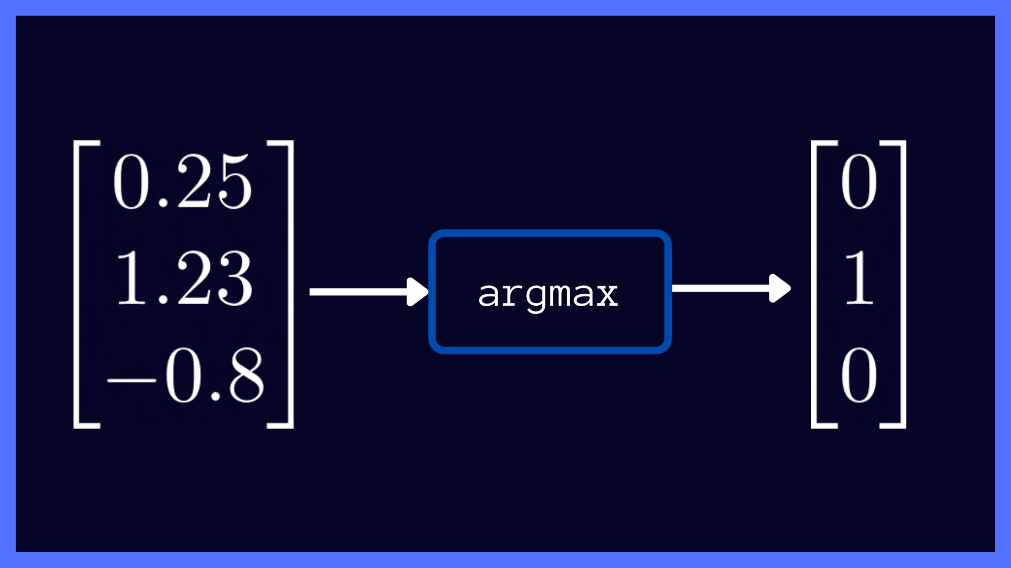
Argmax Output (Image by the author)

One limitation with using the argmax function is that its gradients with respect to the raw outputs of the neural networks are always zero. As you know, it’s the backpropagation of gradients that facilitates the learning process in neural networks.

As you’ll have to plug in the value 0 for all gradients of the argmax output during backpropagation, you cannot use the argmax function in training. Unless there’s backpropagation of gradients, the parameters of the neural network cannot be adjusted, and there’s effectively no learning!

From a probabilistic viewpoint, notice how the argmax function puts all the mass on index 1: the predicted class and 0 elsewhere. So it’s straightforward to infer the predicted class label from the argmax output. However, we would like to know how likely the image is to be that of a panda, a seal, or a duck, and the softmax scores help us with just that!

The Softmax Activation Function, Explained

It’s finally time to learn about softmax activation. The softmax activation function takes in a vector of raw outputs of the neural network and returns a vector of probability scores.

The equation of the softmax function is given as follows:

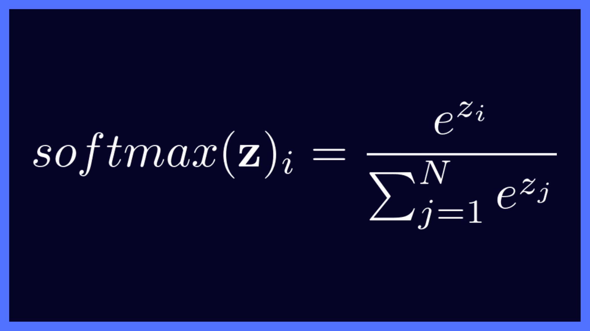
Softmax Function Equation (Image by the author)

Here,

z is the vector of raw outputs from the neural network
The value of e ≈ 2.718
The i-th entry in the softmax output vector softmax(z) can be thought of as the predicted probability of the test input belonging to class i.

From the plot of e^x, you can see that, regardless of whether the input x is positive, negative, or zero, e^x is always a positive number.

Plot of expx
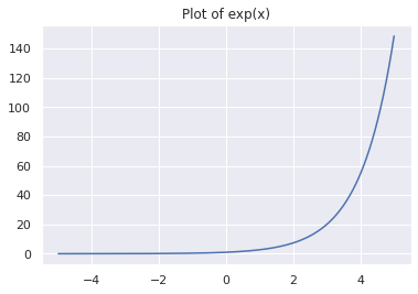
Plot of exp(x)

Recall that in our example, N = 3 as we have 3 classes: {seal, panda, duck}, and the valid indices are 0, 1, and 2. Suppose you’re given the vector z = [0.25, 1.23, -0.8] of raw outputs from the neural network.

Let’s apply the softmax formula on the vector z, using the steps below:

Calculate the exponent of each entry.
Divide the result of step 1 by the sum of the exponents of all entries.

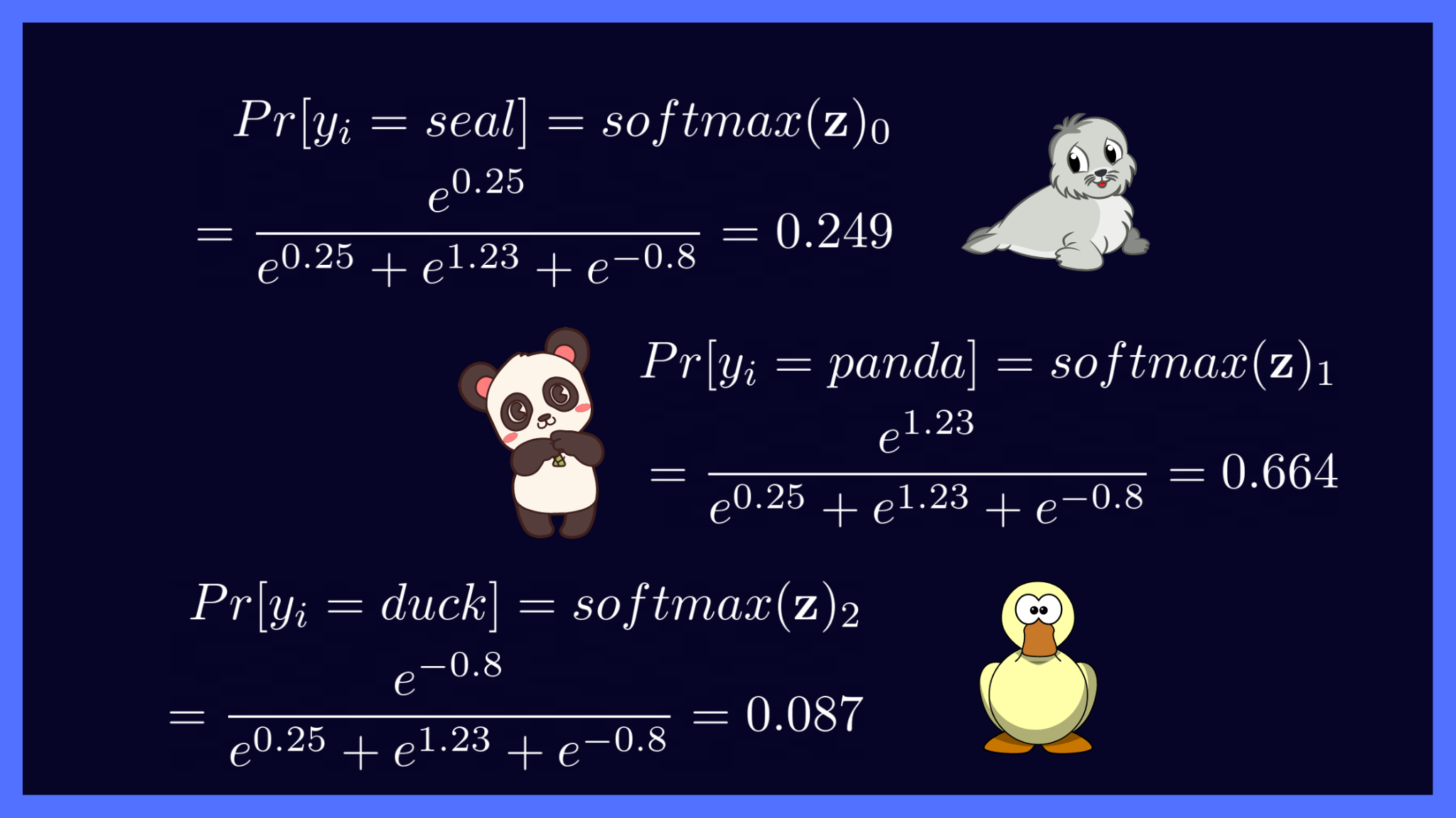
Computing softmax scores for the 3 classes (Image by the author)

▶️ Now that we’ve computed the softmax scores, let’s collect them into a vector for succinct representation, as shown below:

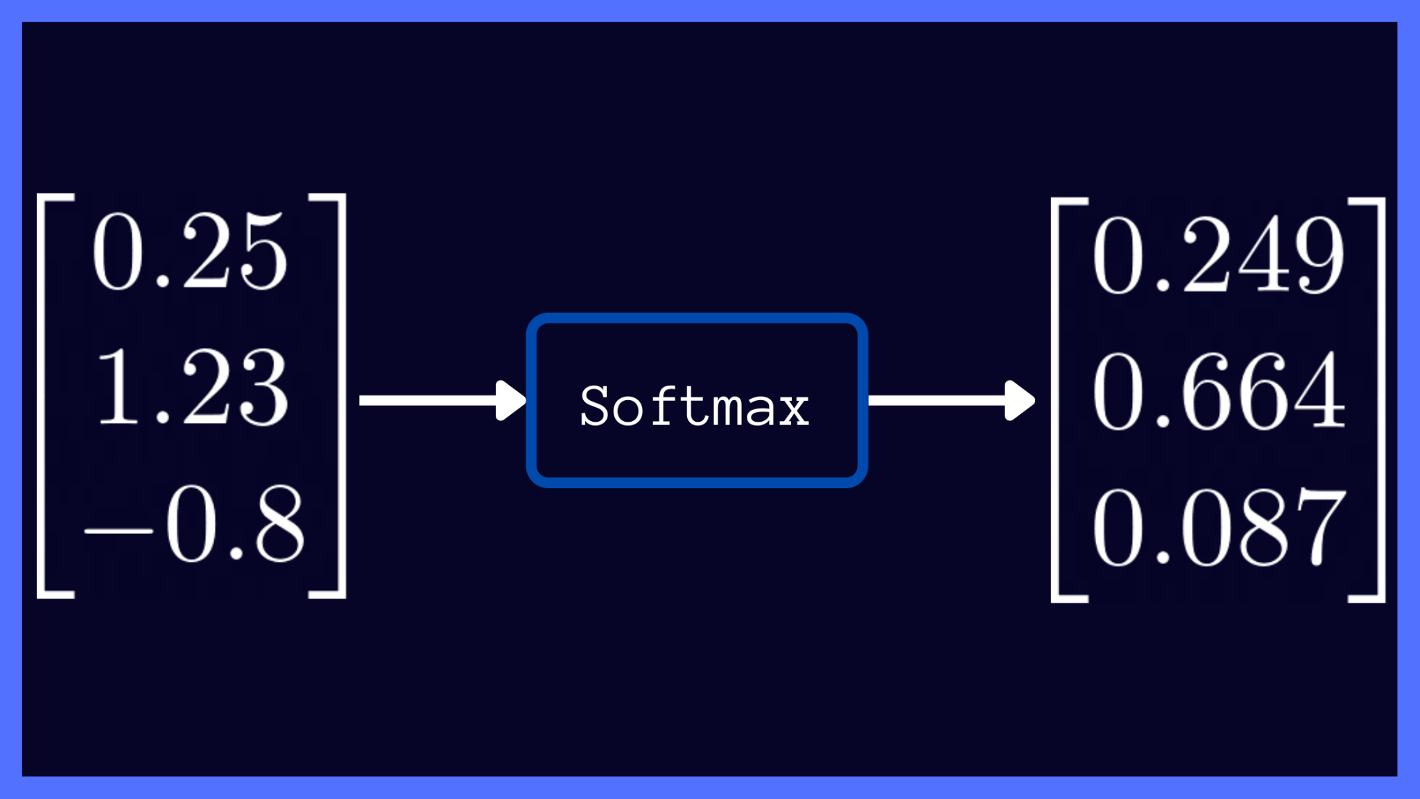
Softmax Output (Image by the author)

From the softmax output above, we can make the following observations:

In the vector z of raw outputs, the maximum value is 1.23, which on applying softmax activation maps to 0.664: the largest entry in the softmax output vector. Likewise, 0.25 and -0.8 map to 0.249 and 0.087: the second and the third largest entries in the softmax output respectively. Thus, applying softmax preserves the relative ordering of scores.
All entries in the softmax output vector are between 0 and 1.
In a multiclass classification problem, where the classes are mutually exclusive, notice how the entries of the softmax output sum up to 1: 0.664 + 0.249 + 0.087 = 1.

This is exactly why you can think of softmax output as a probability distribution over the input classes, that makes it readily interpretable.

As a next step, let’s examine the softmax output for our example.

In the vector softmax(z) = [0.664, 0.294, 0.087], 0.664 at index 1 is the largest value. This means there’s a 66.4% chance that the given image belongs to class 1, which from our one-hot encoding is a class panda.

And the input image has a 29.4% chance of being a seal and around 8.7% chance of being a duck.

Therefore, applying softmax gives instant interpretability, as you know how likely the test image is to belong to each of the 3 classes. In this particular example, it’s highly likely to be a panda and least likely to be a duck.

It now makes sense to call the argmax function on the softmax output to get the predicted class label. As the predicted class label is the one with the highest probability score, you can use argmax(softmax(z)) to obtain the predicted class label. In our example, the highest probability score of 0.664 occurs at index 1, corresponding to class 1 (panda).

How to Implement the Softmax Activation in Python

In the previous section, we did some simple math to compute the softmax scores for the output vector z.

Now let’s translate the math operations into equivalent operations on NumPy arrays. You may use the following code snippet to get the softmax activation for any vector z.

import
 numpy as np

def
 softmax(z):
  '''Return the softmax output of a vector.'''
  exp_z =
 np.exp(z)
  sum =
 exp_z.sum()
  softmax_z =
 np.
round(exp_z/
sum,3)
  return softmax_z

We can parse the definition of the softmax function:

The function takes in one required parameter z, a vector, and returns the softmax output vector softmax_z.
We use np.exp(z) to compute exp(z) for each z in z; call the resultant array exp_z.
Next, we call sum on the array exp_z to compute the sum of exponents.
We then divide each entry in exp_z by the sum and round off the result to 3 decimal places, storing the result in a variable, say, softmax_z.
Finally, the function returns the array softmax_z.

You may now call the function with the output array z as the argument and verify that the scores are identical to what we had computed manually.

z =
 [0.25
, 1.23
, -
0.8]
softmax(z)

# Output
array([ 0.249
, 0.664
, 0.087])

Are you wondering if normalizing each value by the sum of entries will suffice, to get relative scores? Let’s see why it’s not an efficient solution.

Why Won’t Normalization by the Sum Suffice

Why use something math-heavy as the softmax activation? Can we not just divide each of the output values by the sum of all outputs?

Well, let’s try to answer this by taking a few examples.

Use the following function to return the array normalized by the sum.

def
 div_by_sum(z):
  sum_z =
 np.sum(z)
  out_z =
 np.
round(z/
sum_z,3)
  return out_z

1️⃣ Consider z1 = [0.25, 1.23, -0.8], and call the function div_by_sum. In this case, though the entries in the returned array sum up to 1, it has both positive and negative values. We still aren’t able to interpret the entries as probability scores.

z1 =
 [0.25
,1.23
,-
0.8]
div_by_sum(z1)

# Output
array([ 0.368
,  1.809
, -
1.176])

2️⃣ Let z2 = [-0.25, 1, -0.75]. In this case, all elements in the vector sum up to zero, so the denominator will always be 0. When you divide by the sum to normalize, you’ll face runtime warnings, as division by zero is not defined.

z2 =
 [-
0.25
,1
,-
0.75]
div_by_sum(z2)

# Output
RuntimeWarning
: divide by zero encountered in true_divide
array([-
inf,  inf, -inf])

3️⃣ In this example, z3 = [0.1, 0.9, 0.2]. Let’s check both the softmax and normalized scores.

z3 =
 [0.1
,0.9
,0.2
] # ratio: 1:9:2
print(div_by_sum(z3))
print(softmax(z3))

# Output
[0.083
 0.75
  0.167
] # ratio: 1:9:2
[0.231
 0.514
 0.255]

As shown in the code cell above, when all the inputs are positive, you may interpret the normalized scores as probability scores, but the scores are in the same ratio as in the array z3. In this example, the predicted class is still that of a panda.

However, you can’t guarantee that the neural network’s raw output won’t sum up to 0 or have negative entries.

4️⃣ In this example, z4 = [0, 0.9, 0.1]. Let’s check both the softmax and normalized scores.

z4 =
 [0
,0.9
,0.1]
print(div_by_sum(z4))
print(softmax(z4))

# Output
[0.
  0.9
 0.1]
[0.219
 0.539
 0.242]

As you can see, when one of the entries is 0, upon calling the div_by_sum function, the entry is still 0 in the normalized array. However, in the softmax output, you can see that 0 has been mapped to a score of 0.219.

In some sense you can think of the softmax activation function as a softer version of the argmax function: It maximizes the probability score corresponding to the predicted output label. At the same time, it’s soft because it does assign some probability mass to the less likely classes as well, unlike the argmax function that puts the entire probability mass of 1 on the maximum, and 0 everywhere else.

In essence, the softmax activation can be perceived as a smooth approximation to the argmax function.

Equivalence of the Sigmoid, Softmax Activations for N = 2

Now let’s revisit our earlier claim that the sigmoid and softmax activations are equivalent for binary classification when N = 2.

Recall that in binary classification, you apply the sigmoid function to the neural network’s output to get a value in the range [0, 1].

When you’re using the softmax function for multiclass classification, the number of nodes in the output layer = the number of classes N.

You can think of binary classification as a special case of multiclass classification. Assume that the output layer has two nodes: one outputting the score z and the other 0.

Effectively, there’s only one node as the other is not given any weight at all. The raw output vector now becomes z = [z, 0]. Next, we may go ahead and apply softmax activation on this vector z and check how it’s equivalent to the sigmoid function we looked at earlier.

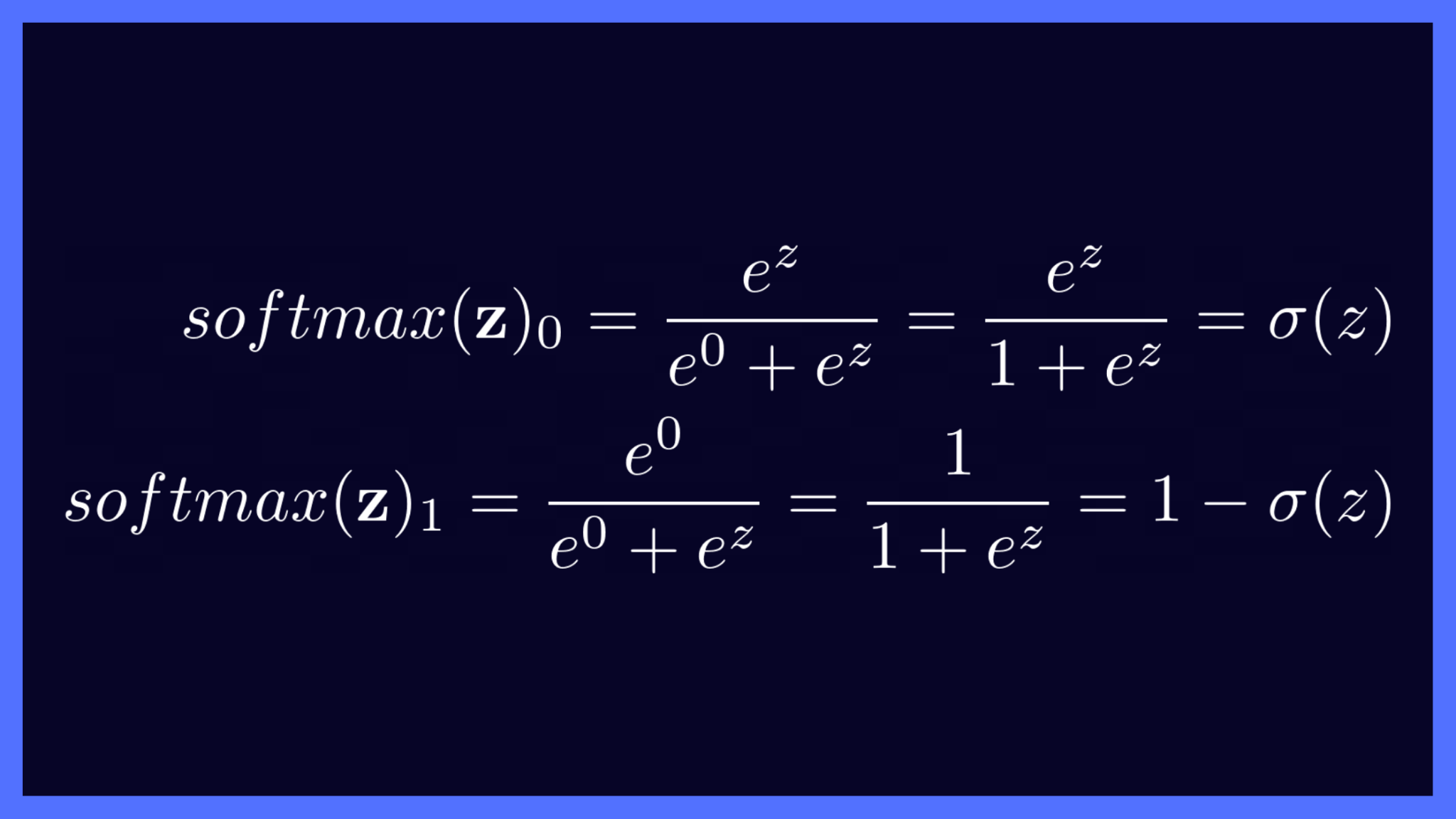
Equivalence of Sigmoid & Softmax Activations (Image by the author)

Observe how the softmax activation scores in this case are the same as the sigmoid activation scores: σ(z) and 1 – σ(z).

And with this, we wrap up our discussion on the softmax activation function. Let’s quickly summarize all that we’ve learned.

Summing Up

In this tutorial, you’ve learned the following:

How to use the softmax function as output layer activation in a multiclass classification problem.
The working of the softmax function—how it transforms a vector of raw outputs into a vector of probabilities. And how you can interpret each entry in the softmax output as the probability of the corresponding class.
How to interpret the softmax activation as an extension of the sigmoid function to multiclass classification, and their equivalence for binary classification where the number of classes N = 2.

In the next tutorial, we’ll delve deep into cross-entropy loss—a widely-used metric to assess how well your multiclass classification model performs.

Until then, check out other interesting NLP tutorials on vector search, algorithms, and more. Happy learning!

Don’t fill this out if you’re human:

Subscribe for more deep learning tutorials!

Subscribed successfully.

Failed to submit.