Perceptrons: The First Neural Networks for Machine Learning

You authorize us to send you information about our products. To learn more please refer to our Privacy Policy

Machine learning is not only a fascinating topic but one with a variety of approaches. Neural networks, one such approach, have come to the forefront largely due to their accessibility for those taking their first step into the machine learning world.

In this tutorial, we’re going to use Python and NumPy to explore the fundamentals of creating neural networks and combining them – using analogies for how our brains work to better understand them.

If you’re ready to start diving deep into the world of machine learning, let’s get started!

Intro & Project Files

Neural Networks have become incredibly popular over the past few years, and new architectures, neuron types, activation functions, and training techniques pop up all the time in research. But without a fundamental understanding of neural networks, it can be quite difficult to keep up with the flurry of new work in this area.

To understand the modern approaches, we have to understand the tiniest, most fundamental building block of these so-called deep neural networks: the neuron. In particular, we’ll see how to combine several of them into a layer and create a neural network called the perceptron. We’ll write Python code (using NumPy) to build a perceptron network from scratch and implement the learning algorithm.

For the completed code, download the ZIP file here.

BUILD GAMES

FINAL DAYS: Unlock 250+ coding courses, guided learning paths, help from expert mentors, and more.

ACCESS NOW

Biological Neurons

Perceptrons and artificial neurons actually date back to 1958. Frank Rosenblatt was a psychologist trying to solidify a mathematical model for biological neurons. To better understand the motivation behind the perceptron, we need a superficial understanding of the structure of biological neurons in our brains.

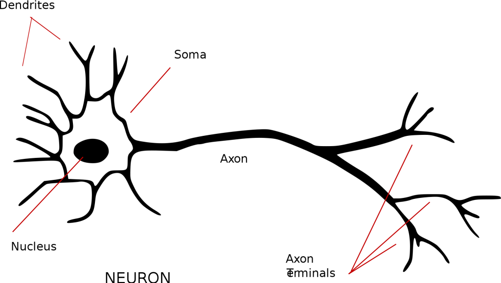
(Credit: https://commons.wikimedia.org/wiki/File:Neuron_-_annotated.svg)

Let’s consider a biological neuron. The point of this cell is to take in some input (in the form of electrical signals in our brains), do some processing, and produce some output (also an electrical signal). One very important thing to note is that the inputs and outputs are binary (0 or 1)! An individual neuron accepts inputs, usually from other neurons, through its dendrites. Although the image above doesn’t depict it, the dendrites connect with other neurons through a gap called the synapse that assigns a weight to a particular input. Then, all of these inputs are considered together when they are processed in the cell body, or soma.

Neurons exhibit an all-or-nothing behavior. In other words, if the combination of inputs exceeds a certain threshold, then an output signal is produced, i.e., the neuron “fires.” If the combination falls short of the threshold, then the neuron doesn’t produce any output, i.e., the neuron “doesn’t fire.” In the case where the neuron does fire, the output travels along the axon to the axon terminals. These axon terminals are connected to the dendrites of other neurons through the synapse.

Let’s take a moment to recap biological neurons. They take some binary inputs through the dendrites, but not all inputs are treated the same since they are weighted. We combine these weighted signals and, if they surpass a threshold, the neuron fires. This single output travels along the axon to other neurons. Now that we have this summary in mind, we can develop mathematical equations to roughly represent a biological neuron.

Artificial Neurons

Now that we have some understanding of biological neurons, the mathematical model should follow from the operations of a neuron.

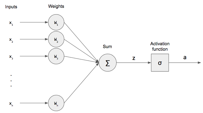
In this model, we have n binary inputs (usually given as a vector) and exactly the same number of weights $W_1, …, W_n$. We multiply these together and sum them up. We denote this as z and call it the pre-activation.

\[ z = \displaystyle\sum_{i=1}^{n} W_i x_i = W^T x \]

(We can re-write this as an inner product for succinctness.) There is another term, called the bias, that is just a constant factor.

\[ z = \displaystyle\sum_{i=1}^{n} W_i x_i + b = W^T x + b \]

For mathematical convenience, we can actually incorporate it into our weight vector as $W_0$ and set $x_0 = +1$ for all of our inputs. (This concept of incorporating the bias into the weight vector will become clearer when we write code.)

\[ z = \displaystyle\sum_{i=0}^{n} W_i x_i = W^T x \]

After taking the weighted sum, we apply an activation function, $\sigma$, to this and produce an activation a. The activation function for perceptrons is sometimes called a step function because, if we were to plot it, it would look like a stair.

\[
\sigma(q)=
\begin{cases}
1 & q\geq 0 \\
0 & q < 0
\end{cases}
\]

In other words, if the input is greater than or equal to 0, then we produce an output of 1. Otherwise, we produce an output of 0. This is the mathematical model for a single neuron, the most fundamental unit for a neural networks.

\[ a = \sigma (W^T x) \]

Let’s compare this model to the biological neuron. The inputs are analogous to the dendrites, and the weights model the synapse. We combine the weighted inputs by summing and send that weighted sum to the activation function. This acts as our all-or-nothing response function where 0 means the neuron didn’t produce an output. Also note that our inputs and outputs are also binary, which is in accordance with the biological model.

Capabilities and Limitations of Perceptrons

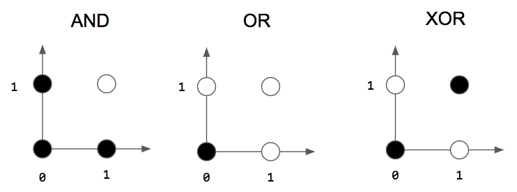
Since the output of a perceptron is binary, we can use it for binary classification, i.e., an input belongs to only one of two classes. The classic examples used to explain what perceptrons can model are logic gates!

Let’s consider the logic gates in the figure above. A white circle means an output of 1 and a black circle means an output of 0, and the axes indicate inputs. For example, when we input 1 and 1 to an AND gate, the output is 1, the white circle. We can create perceptrons that act like gates: they take 2 binary inputs and produce a single binary output!

However, perceptrons are limited to solving problems that are linearly separable. If two classes are linearly separable, this means that we can draw a single line to separate the two classes. We can do this easily for the AND and OR gates, but there is no single line that can separate the classes for the XOR gate! This means that we can’t use our single-layer perceptron to model an XOR gate.

An intuitive way to understand why perceptrons can only model linearly separable problems is to look the weighted sum equation (with the bias).

\[ \displaystyle\sum_{i=0}^N W_i x_i + b \]

This looks very similar to the equation of a line! (Or, more generally, a hyperplane.) Hence, we’re creating a line and saying that everything on one side of the line belongs to one class and everything on the other side belongs to the other class. This line is called the decision boundary, and, when we use a single-layer perceptron, we can only produce one decision boundary.

In light of this new information, it doesn’t seem like perceptrons are useful! But, in practice, many problems are actually linearly separable. Hope is not lost for non-linearly separably problems however! It can be shown that organizing multiple perceptrons into layers and using an intermediate layer, or hidden layer, can solve the XOR problem! This is the foundation of modern neural networks!

Single-Layer Perceptron Code

Now that we have a good understanding of how perceptrons works, let’s take one more step and solidify the math into code. We’ll use object-oriented principles and create a class. In order to construct our perceptron, we need to know how many inputs there are to create our weight vector. The reason we add one to the input size is to include the bias in the weight vector.

import numpy as np

class Perceptron(object):
    """Implements a perceptron network"""
    def __init__(self, input_size):
        self.W = np.zeros(input_size+1)

We’ll also need to implement our activation function. We can simply return 1 if the input is greater than or equal to 0 and 0 otherwise.

def activation_fn(self, x):
    return 1 if x >= 0 else 0

Finally, we need a function to run an input through the perceptron and return an output. Conventionally, this is called the prediction. We add the bias into the input vector. Then we can simply compute the inner product and apply the activation function.

def predict(self, x):
    x = np.insert(x, 0, 1)
    z = self.W.T.dot(x)
    a = self.activation_fn(z)
    return a

All of these are functions of the Perceptron class that we’ll use for perceptron learning.

Perceptron Learning Algorithm

We’ve defined a perceptron, but how do perceptrons learn? Rosenblatt, the creator of the perceptron, also had some thoughts on how to train neurons based on his intuition about biological neurons. Rosenblatt intuited a simple learning algorithm. His idea was to run each example input through the perceptron and, if the perceptron fires when it shouldn’t have, inhibit it. If the perceptron doesn’t fire when it should have, excite it.

How do we inhibit or excite? We change the weight vector (and bias)! The weight vector is a parameter to the perceptron: we need to keep changing it until we can correctly classify each of our inputs. With this intuition in mind, we need to write an update rule for our weight vector so that we can appropriately change it:

\[ w \leftarrow w + \Delta w \]

We have to determine a good $\Delta w$ that does what we want. First, we can define the error as the difference between the desired output d and the predicted output y.

\[ e = d – y \]

Notice that when d and y are the same (both are 0 or both are 1), we get 0! When they are different, (0 and 1 or 1 and 0), we can get either 1 or -1. This directly corresponds to exciting and inhibiting our perceptron! We multiply this with the input to tell our perceptron to change our weight vector in proportion to our input.

\[ w \leftarrow w + \eta\cdot e\cdot x \]

There is a hyperparameter $\eta$ that is called the learning rate. It is just a scaling factor that determines how large the weight vector updates should be. This is a hyperparameter because it is not learned by the perceptron (notice there’s no update rule for $\eta$!), but we select this parameter.

(For perceptrons, the Perceptron Convergence Theorem says that a perceptron will converge, given that the classes are linearly separable, regardless of the learning rate. But for other learning algorithms, this is a critical parameter!)

Let’s take another look at this update rule. When the error  is 0, i.e., the output is what we expect, then we don’t change the weight vector at all. When the error is nonzero, we update the weight vector accordingly.

Perceptron Learning Algorithm Code

With the update rule in mind, we can create a function to keep applying this update rule until our perceptron can correctly classify all of our inputs. We need to keep iterating through our training data until this happens; one epoch is when our perceptron has seen all of the training data once. Usually, we run our learning algorithm for multiple epochs.

Before we code the learning algorithm, we need to make some changes to our init function to add the learning rate and number of epochs as inputs.

def __init__(self, input_size, lr=1, epochs=10):
    self.W = np.zeros(input_size+1)
    # add one for bias
    self.epochs = epochs
    self.lr = lr

Now we can create a function, given inputs and desired outputs, run our perceptron learning algorithm. We keep updating the weights for a number of epochs, and iterate through the entire training set. We insert the bias into the input when performing the weight update. Then we can create our prediction, compute our error, and perform our update rule.

def fit(self, X, d):
    for _ in range(self.epochs):
        for i in range(d.shape[0]):
            y = self.predict(X[i])
            e = d[i] - y
            self.W = self.W + self.lr * e * np.insert(X[i], 0, 1)

The entire code for our perceptron is shown below.

class Perceptron(object):
    """Implements a perceptron network"""
    def __init__(self, input_size, lr=1, epochs=100):
        self.W = np.zeros(input_size+1)
        # add one for bias
        self.epochs = epochs
        self.lr = lr
    
    def activation_fn(self, x):
        #return (x >= 0).astype(np.float32)
        return 1 if x >= 0 else 0

    def predict(self, x):
        z = self.W.T.dot(x)
        a = self.activation_fn(z)
        return a

    def fit(self, X, d):
        for _ in range(self.epochs):
            for i in range(d.shape[0]):
                x = np.insert(X[i], 0, 1)
                y = self.predict(x)
                e = d[i] - y
                self.W = self.W + self.lr * e * x

Now that we have our perceptron coded, we can try to give it some training data and see if it works! One easy set of data to give is the AND gate. Here’s a set of inputs and outputs.

if __name__ == '__main__':
    X = np.array([
        [0, 0],
        [0, 1],
        [1, 0],
        [1, 1]
    ])
    d = np.array([0, 0, 0, 1])

    perceptron = Perceptron(input_size=2)
    perceptron.fit(X, d)
    print(perceptron.W)

In just a few lines, we can start using our perceptron! At the end, we print the weight vector. Using the AND gate data, we should get a weight vector of [-3, 2, 1]. This means that the bias is -3 and the weights are 2 and 1 for $x_1$ and $x_2$, respectively.

To verify this weight vector is correct, we can try going through a few examples. If both inputs are 0, then the pre-activation will be -3+0*2+0*1 = -3. When applying our activation function, we get 0, which is exactly 0 AND 0! We can try this for other gates as well. Note that this is not the only correct weight vector. Technically, if there exists a single weight vector that can separate the classes, there exist an infinite number of weight vectors. Which weight vector we get depends on how we initialize the weight vector.

To summarize, perceptrons are the simplest kind of neural network: they take in an input, weight each input, take the sum of weighted inputs, and apply an activation function. Since they were modeled from biological neurons by Frank Rosenblatt, they take and produce only binary values. In other words, we can perform binary classification using perceptrons. One limitation of perceptrons is that they can only solve linearly separable problems. In the real world, however, many problems are actually linearly separable. For example, we can use a perceptron to mimic an AND or OR gate. However, since XOR is not linearly separable, we can’t use single-layer perceptrons to create an XOR gate. The perceptron learning algorithm fits the intuition by Rosenblatt: inhibit if a neuron fires when it shouldn’t have, and excite if a neuron does not fire when it should have. We can take that simple principle and create an update rule for our weights to give our perceptron the ability of learning.

Perceptrons are the foundation of neural networks so having a good understanding of them now will be beneficial when learning about deep neural networks! This will also help as you pursue exciting developer opportunities.

Want to learn more Python in general? Check out our free course on Kivy!

Related Posts