How to build a convolutional neural network in Keras – Ander Fernández

Treating images using convolutional neural networks with Keras

Convolutional neural networks apply neural networks on images. On pictures? Yes, with them you can classify images, detect what they contain, generate new images … all this is possible thanks to convolutional neural networks. In this post I am going to explain what they are and how you can create a convolutional neural network in Keras with Python. Sounds interesting right? Well let’s get to it!

From images to numbers

One of the first questions we usually ask ourselves when faced with this problem is, how can we work on an image? Well, the first thing to do is to turn images it into numbers. I explain you how.

Let’s think of a monochrome image (one that has black or white colors). If you think about it, an image is no more than many pixels (little squares) together. Each of those pixels store information. In the case of monochrome images, for example, the pixel stores two values: 1 if it is white and 0 if it is black (or vice versa).

So if you think about it, a monochrome image is nothing more than a large dataset of ones and zeros. But what about color images?Inkabet apuestas en vivo

Well, the logic behind is the same, only in this case, there is not a single layer, but three: a red (R), a green (G) and a blue (B). RGB. Sounds familiar? I suppose so since RGB is the color composition of most screen images.

Composition of an image with RGB layers

With that being said, let’s see how we can read images, in this case in Python.

Reading Images in Python

The theory is fine but without practice … it is useless. So, let’s see how to create an image classifier that classifies between cats and dogs. To do this, the dataset I’m going to use is Kaggle’s Cat vs Dog dataset. As the information is a zip file, first I unzip the global zip and then another one of the train.zip file.

import os
from zipfile import ZipFile

with ZipFile('dogs-vs-cats.zip', 'r') as zipObj:
   # Extract all the contents of zip file in current directory
   zipObj.extractall()

with ZipFile('train.zip', 'r') as zipObj:
   # Extract all the contents of zip file in current directory
   zipObj.extractall()

Now we are going to create a data frame with each of the objects within the folder that we have downloaded. Whether the image is a cat or a dog is indicated on the name of the image. Thus, we will need to extract that info.

import pandas as pd 

filenames = os.listdir("train")

categories = []
for filename in filenames:
    category = filename.split('.')[0]
    if category == 'dog':
        categories.append(1)
    else:
        categories.append(0)

df = pd.DataFrame({
    'filename': filenames,
    'category': categories
})

df.head(5)

filenamecategory0cat.0.jpg01cat.1.jpg02cat.10.jpg03cat.100.jpg04cat.1000.jpg0

As you can see we just have a dataframe with the file name and their label. Now we can open that file so that you can see what Python really reads when we read an image: a three dimensional array with values between 0 an 250. These numbers are the limits of RGB colors.

import matplotlib.pyplot as plt
import matplotlib.image as mpimg

img=mpimg.imread('train/cat.0.jpg')
img

array([[[203, 164,  87],
        [203, 164,  87],
        [204, 165,  88],
        ...,
        [240, 201, 122],
        [239, 200, 121],
        [238, 199, 120]],

       [[203, 164,  87],
        [203, 164,  87],
        [204, 165,  88],
        ...,
        [241, 202, 123],
        [240, 201, 122],
        [238, 199, 120]],

       [[203, 164,  87],
        [203, 164,  87],
        [204, 165,  88],
        ...,
        [241, 202, 123],
        [240, 201, 122],
        [239, 200, 121]],

       ...,

       [[153, 122,  55],
        [153, 122,  55],
        [153, 122,  55],
        ...,
        [  2,   2,   0],
        [  2,   2,   0],
        [  2,   2,   0]],

       [[152, 121,  54],
        [152, 121,  54],
        [152, 121,  54],
        ...,
        [  2,   2,   0],
        [  2,   2,   0],
        [  2,   2,   0]],

       [[151, 120,  53],
        [151, 120,  53],
        [151, 120,  53],
        ...,
        [  1,   1,   0],
        [  1,   1,   0],
        [  1,   1,   0]]], dtype=uint8)

If we plot all those numbers as color layers, what we will see is the picture of a cat:

plt.imshow(img) 

<matplotlib.image.AxesImage at 0x1bc258c1b38>

Understanding what a convolutional neural network is

We have just learned how to read an image. Now we could transform the arrays we have seen from three dimensional to one dimensional. By doing so, we could build a fully connected neural network, as we did on this post with Tensorlow or at this from scratch, both in R.

Despite this approach is possible, it is feasible as fully connected layers are not very efficient for working with images. Convolutional neural networks, on the other hand, are much more suited for this job.

Convolutional neural networks basically take an image as input and apply different transformations that condense all the information. These processes are the following:

Convolutional Layer

This layers convolves an image by a matrix, called Kerner or filter. The proccess is as follows:

1. First, you overlay the kernel onto the image.
2. Then you multiply the kernel value by the image value.
3. After that, you calculate the product of the results of the previous step.
4. Finally, you move the kernel one pixel and repeat the process.

This is a very visual example of how a convolutional layer works:

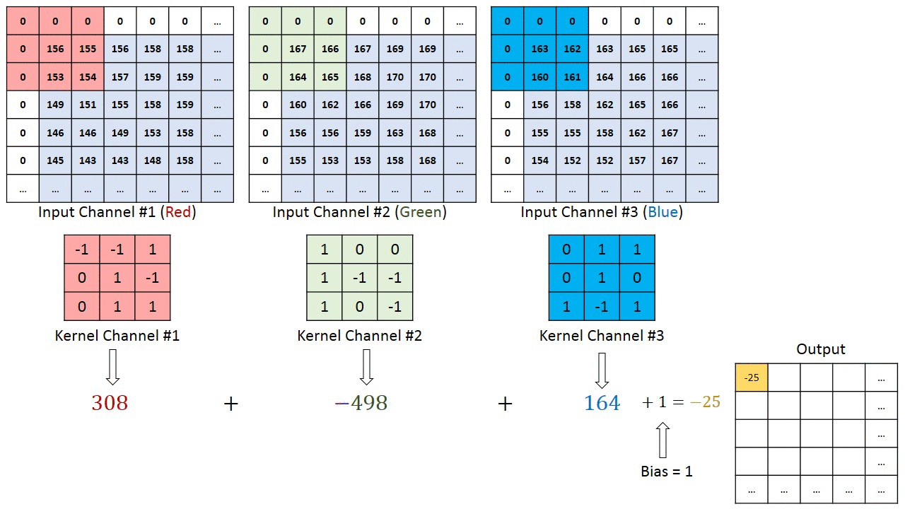
Once we have the result from the previous step, we will do as we do on fully connected layers: we add the bias parameter and then apply an activation function. If you want to learn more about activation functions, check this post where I code them from scratch. I will even so you how to code them;)

Thanks to convolutional layers, our neural network is able to detect lines, forms, textures and many things. If you don’t believe me, try doing the convolution of this image from Deeplearning.ai:

Despite being an easy step, most certainly you will have many doubts right now, such as:

• Which dimensions should the Kernel have?
• Which values?
• How can I create a convolutional layer?
• If with every layer we get smaller results… is there any maximum amount of layers that we can apply?

Let’s answer those questions one by one.

Which dimensions should the Kernel have?

Despite there is not ‘one size fits all’ Kernel, neural networks with more layers and smaller kernels are more efficient that neural networks with less layers and bigger Kernels (link). In fact, most kernels have a dimension of 3 by 3 (link).

Conclusion: most probably 3 by 3 Kernels will work fine.

Which values should the Kernel of the convolutional neural network have?

Despite some Kernel structures can identify different shapes, Kernel values are usually set as parameters that the neural network should optimize. By doing so, we ensure that neural network applies the best possible Kernels for that specific dataset.

Conclusion: Kernel values will be randomly initialized and will be optimized by the neural network.

How can I build a convolutional layer?

You can build a neural very easily with either Tensorflow or Keras.

• Tensorflow: tf.nn.conv2d()
• Keras: model.add(layers.Conv2D())

Is there a limit to the amount of convolutional layers that we can have?

As you have guessed, with every convolutional layer the size of the result is smaller than the input of the layer. Thus, if we just apply convolutional layers with no other changes, yes, there is a maximum amount of layers that we can apply.

Anyway, we can add a padding to the image so that the result of the image does not reduce in size.

The padding basically consists of adding some pixels on the borders of the image before applying the convolution. By doing so, we can get a result that has the same size as the input (without the padding).

Besides, padding is very easy to set in frameworks like Keras or Tensorflow, as it is basically a parameter that needs to be set on a function. We will see this later.

Pooling Layers

As we have learned, convolutional layers enable to detect shapes on an image keeping the image size. However, big images imply more work and slower and more difficult trainings, so we might want to reduce the size of the image at any time. Pooling layers will help us do so.

Pooling layers allow us to reduce the size of the image so that the neural network works faster. It basically creates a smaller image by dividing the image in several n by n matrices (say 2 by 2 matrices).

Depending on the type of pooling layer, the way of calculating the result might vary. In Max Pooling layers, for example, the result will be the maximum value of each smaller matrix. In Average Layers, on the other hand, the result will be the average of the smaller matrix. Let’s see an example of a Max Pooling layer:

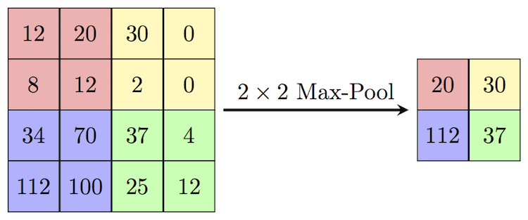
By applying a max pooling layer we ensure that the shapes detected by the convolutional layer are maintained for the next layer. Because of this, Max Pooling layers are the most used pooling layers, as they are they usually give better results.

Finally, pooling layers do not have any trainable parameters, and we can apply it as follows:

• Tensorflow: tf.nn.max_pool2d()
• Keras: tf.keras.layers.MaxPool2D()

With all this theoretical introduction, we can now dive into coding our convolutional neural network in Keras. Let’s go!

Building a Convolutional Neural Network in Keras

Building our network’s structure

Considering all the above, we will create a convolutional neural network that has the following structure:

1. One convolutional layer with a 3×3 Kernel and no paddings followed by a MaxPooling of 2 by 2.
2. Another convolutional layer with a 3 by 3 Kernel and no paddings followe by a MaxPooling 2 by 2 layer.
3. A flattening layer so that we can make a prediction.

Let’s get it done!

from keras.layers import Conv2D, MaxPooling2D, Flatten, Dense
from keras.models import Sequential

model = Sequential()

# Añadimos la primera capa
model.add(Conv2D(64,(3,3), activation = 'relu', input_shape = (128,128,3)))
model.add(MaxPooling2D(pool_size = (2,2)))

# Añadimos la segunda capa
model.add(Conv2D(64,(3,3), activation = 'relu'))
model.add(MaxPooling2D(pool_size = (2,2)))

# Hacemos un flatten para poder usar una red fully connected
model.add(Flatten())
model.add(Dense(64, activation='relu'))

# Añadimos una capa softmax para que podamos clasificar las imágenes
model.add(Dense(2, activation='softmax'))


model.compile(optimizer="rmsprop",
              loss='categorical_crossentropy',
              metrics=['accuracy'])

That’s it! We have just created the structure of our network. Now, let’s see how we prepare the data and train the model.

Preparing the data for our model

Now that we have build our model we will:

• Convert the label into 0 or 1.
• Create the train and test dataframe.
• Generate batches and apply data augmentation to improve performance on new images (that to Usimity’s notebook).

As you can see the first two steps are very similar to what we would do on a fully connected neural network. The thirds step, the data augmentation step, however, is something new.

An image is a very big array of numbers. So, if we deal with big images, we will need a lot of memory to store all that information and do all the math. However, we don’t always have that much memory available in our computer. Thus, in order to make the training process feasible, we break the trainig process in smaller sets known as batches.

Besides, we can apply different distortions to our images (zoom, flip, etc.) so that we can increase the number of images in our dataset. This is a good way of increasing performance in a simple way and it can be done using the ImageDataGenerator function in Keras.

from sklearn.model_selection import train_test_split
from keras.preprocessing.image import ImageDataGenerator

# We convert the variable in dog or cat
df["category"] = df["category"].replace({0: 'gato', 1: 'perro'})

# We create the split
df_train, df_test = train_test_split(df, test_size=0.25, random_state=42)

# We apply some modifications to get more images
datos_train = ImageDataGenerator(
    rotation_range=15,
    rescale=1./255,        # We normalize the image
    shear_range=0.1,
    zoom_range=0.2,
    horizontal_flip=True,
    width_shift_range=0.1,
    height_shift_range=0.1
)

# We generate images
tamaño_batch = 15
generador_train = datos_train.flow_from_dataframe(
    df_train, 
    "train/", 
    x_col='filename',
    y_col='category',
    target_size= (128,128),
    class_mode= 'categorical',
    batch_size= tamaño_batch
)


# We repeat the process for test data
datos_test =  ImageDataGenerator(rescale=1./255)
generador_test = datos_test.flow_from_dataframe(
    df_test, 
    "train/", 
    x_col='filename',
    y_col='category',
    target_size=(128,128),
    class_mode='categorical',
    batch_size=tamaño_batch
)

Found 18750 validated image filenames belonging to 2 classes.
Found 6250 validated image filenames belonging to 2 classes.

Training our convolutional neural network in Keras

Now that we have the data prepared and the structure created we just need to train our model. This might take a while if you train on CPU so, if you can I would recommend training it on GPU either on your computer or on Colab.

epochs=3 
history = model.fit_generator(
    generador_train, 
    epochs=epochs,
    validation_data=generador_test,
    validation_steps=df_test.shape[0]//tamaño_batch,
    steps_per_epoch=df_train.shape[0]//tamaño_batch
)

WARNING:tensorflow:From <ipython-input-8-34fa295a25fe>:7: Model.fit_generator (from tensorflow.python.keras.engine.training) is deprecated and will be removed in a future version.
Instructions for updating:
Please use Model.fit, which supports generators.
WARNING:tensorflow:sample_weight modes were coerced from
  ...
    to  
  ['...']
WARNING:tensorflow:sample_weight modes were coerced from
  ...
    to  
  ['...']
Train for 1250 steps, validate for 416 steps
Epoch 1/3
1250/1250 [==============================] - 516s 413ms/step - loss: 0.6497 - accuracy: 0.6429 - val_loss: 0.5669 - val_accuracy: 0.7091
Epoch 2/3
1250/1250 [==============================] - 403s 322ms/step - loss: 0.5747 - accuracy: 0.7042 - val_loss: 0.5024 - val_accuracy: 0.7591
Epoch 3/3
1250/1250 [==============================] - 396s 317ms/step - loss: 0.5385 - accuracy: 0.7395 - val_loss: 0.5020 - val_accuracy: 0.7505

As we can see, validation accuracy has increased while validation loss keeps reducing. It is obvious that network has trained, but let’s see the results more visually:

import matplotlib.pyplot as plt

acc = history.history['accuracy']
epochs = range(epochs)
plt.plot(epochs, acc)
plt.title('Accuracy evolution')

Text(0.5, 1.0, 'Training and validation loss')

Despite we have trained our model for three epochs we can see how it has improve its performance from a 70% accuracy on the first epoch to the 75% accuracy on the third epoch. Congratulations! You have learned how to build a convolutional neural network in Keras.

I hope you have enjoyed the tutorial. As always, if you have any doubt do not hesitate to contact me on Linkedin. See you on the next post!