Machine learning, and especially deep learning, are two technologies that are changing the world.

After a long “AI winter” that spanned 30 years, computing power and data sets have finally caught up to the artificial intelligence algorithms that were proposed during the second half of the twentieth century.

This means that deep learning models are finally being used to make effective predictions that solve real-world problems.

It’s more important than ever for data scientists and software engineers to have a high-level understanding of how deep learning models work. This article will explain the history and basic concepts of deep learning neural networks in plain English.

The History of Deep Learning

Deep learning was conceptualized by Geoffrey Hinton in the 1980s. He is widely considered to be the founding father of the field of deep learning. Hinton has worked at Google since March 2013 when his company, DNNresearch Inc., was acquired.

Hinton’s main contribution to the field of deep learning was to compare machine learning techniques to the human brain.

More specifically, he created the concept of a “neural network”, which is a deep learning algorithm structured similar to the organization of neurons in the brain. Hinton took this approach because the human brain is arguably the most powerful computational engine known today.

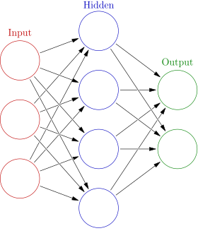
The structure that Hinton created was called an artificial neural network (or artificial neural net for short). Here’s a brief description of how they function:

• Artificial neural networks are composed of layers of node
• Each node is designed to behave similarly to a neuron in the brain
• The first layer of a neural net is called the input layer, followed by hidden layers, then finally the output layer
• Each node in the neural net performs some sort of calculation, which is passed on to other nodes deeper in the neural net

Here is a simplified visualization to demonstrate how this works:

Neural nets represented an immense stride forward in the field of deep learning.

However, it took decades for machine learning (and especially deep learning) to gain prominence.

We’ll explore why in the next section.

Why Deep Learning Did Not Immediately Work

If deep learning was originally conceived decades ago, why is it just beginning to gain momentum today?

It’s because any mature deep learning model requires an abundance of two resources:

• Data
• Computing power

At the time of deep learning’s conceptual birth, researchers did not have access to enough of either data or computing power to build and train meaningful deep learning models. This has changed over time, which has led to deep learning’s prominence today.

Understanding Neurons in Deep Learning

Neurons are a critical component of any deep learning model.

In fact, one could argue that you can’t fully understand deep learning with having a deep knowledge of how neurons work.

This section will introduce you to the concept of neurons in deep learning. We’ll talk about the origin of deep learning neurons, how they were inspired by the biology of the human brain, and why neurons are so important in deep learning models today.

What is a Neuron in Biology?

Neurons in deep learning were inspired by neurons in the human brain. Here is a diagram of the anatomy of a brain neuron:

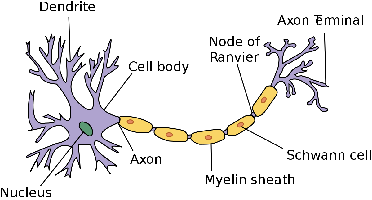
As you can see, neurons have quite an interesting structure. Groups of neurons work together inside the human brain to perform the functionality that we require in our day-to-day lives.

The question that Geoffrey Hinton asked during his seminal research in neural networks was whether we could build computer algorithms that behave similarly to neurons in the brain. The hope was that by mimicking the brain’s structure, we might capture some of its capability.

To do this, researchers studied the way that neurons behaved in the brain. One important observation was that a neuron by itself is useless. Instead, you require networks of neurons to generate any meaningful functionality.

This is because neurons function by receiving and sending signals. More specifically, the neuron’s dendrites receive signals and pass along those signals through the axon.

The dendrites of one neuron are connected to the axon of another neuron. These connections are called synapses, which is a concept that has been generalized to the field of deep learning.

What is a Neuron in Deep Learning?

Neurons in deep learning models are nodes through which data and computations flow.

Neurons work like this:

• They receive one or more input signals. These input signals can come from either the raw data set or from neurons positioned at a previous layer of the neural net.
• They perform some calculations.
• They send some output signals to neurons deeper in the neural net through a synapse.

Here is a diagram of the functionality of a neuron in a deep learning neural net:

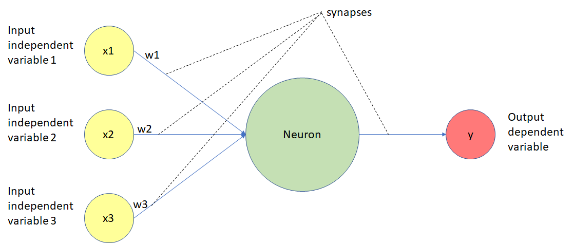
Let’s walk through this diagram step-by-step.

As you can see, neurons in a deep learning model are capable of having synapses that connect to more than one neuron in the preceding layer. Each synapse has an associated weight, which impacts the preceding neuron’s importance in the overall neural network.

Weights are a very important topic in the field of deep learning because adjusting a model’s weights is the primary way through which deep learning models are trained. You’ll see this in practice later on when we build our first neural networks from scratch.

Once a neuron receives its inputs from the neurons in the preceding layer of the model, it adds up each signal multiplied by its corresponding weight and passes them on to an activation function, like this:

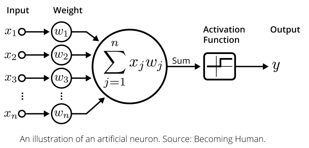
The activation function calculates the output value for the neuron. This output value is then passed on to the next layer of the neural network through another synapse.

This serves as a broad overview of deep learning neurons. Do not worry if it was a lot to take in – we’ll learn much more about neurons in the rest of this tutorial. For now, it’s sufficient for you to have a high-level understanding of how they are structured in a deep learning model.

Deep Learning Activation Functions

Activation functions are a core concept to understand in deep learning.

They are what allows neurons in a neural network to communicate with each other through their synapses.

In this section, you will learn to understand the importance and functionality of activation functions in deep learning.

What Are Activation Functions in Deep Learning?

In the last section, we learned that neurons receive input signals from the preceding layer of a neural network. A weighted sum of these signals is fed into the neuron’s activation function, then the activation function’s output is passed onto the next layer of the network.

There are four main types of activation functions that we’ll discuss in this tutorial:

• Threshold functions
• Sigmoid functions
• Rectifier functions, or ReLUs
• Hyperbolic Tangent functions

Let’s work through these activations functions one-by-one.

Threshold Functions

Threshold functions compute a different output signal depending on whether or not its input lies above or below a certain threshold. Remember, the input value to an activation function is the weighted sum of the input values from the preceding layer in the neural network.

Mathematically speaking, here is the formal definition of a deep learning threshold function:

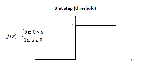
As the image above suggests, the threshold function is sometimes also called a unit step function.

Threshold functions are similar to boolean variables in computer programming. Their computed value is either 1 (similar to True) or 0 (equivalent to False).

The Sigmoid Function

The sigmoid function is well-known among the data science community because of its use in logistic regression, one of the core machine learning techniques used to solve classification problems.

The sigmoid function can accept any value, but always computes a value between 0 and 1.

Here is the mathematical definition of the sigmoid function:

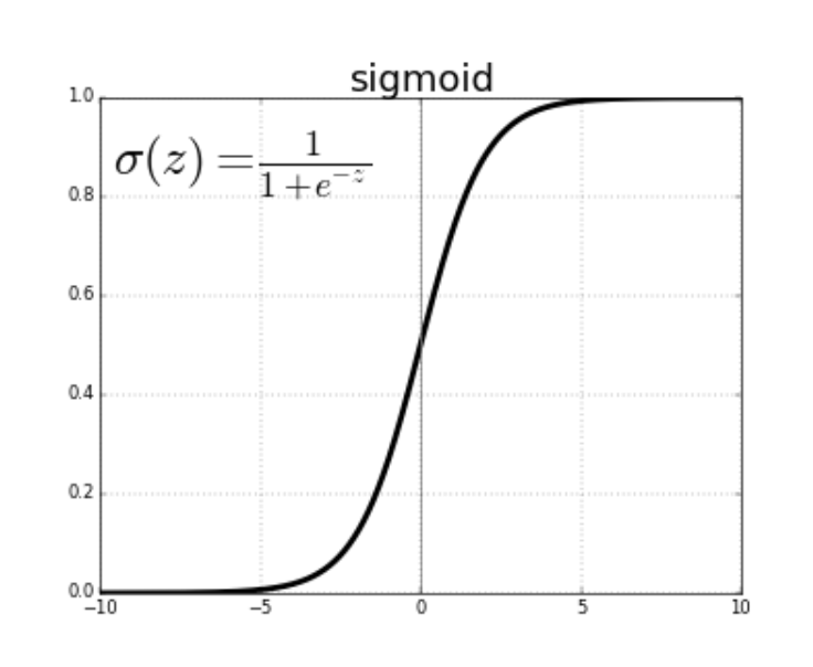
One benefit of the sigmoid function over the threshold function is that its curve is smooth. This means it is possible to calculate derivatives at any point along the curve.

The Rectifier Function

The rectifier function does not have the same smoothness property as the sigmoid function from the last section. However, it is still very popular in the field of deep learning.

The rectifier function is defined as follows:

• If the input value is less than 0, then the function outputs 0
• If not, the function outputs its input value

Here is this concept explained mathematically:

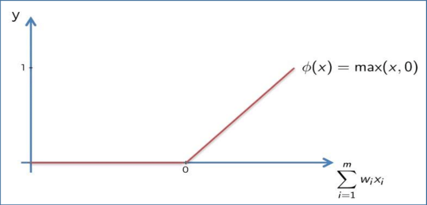
Rectifier functions are often called Rectified Linear Unit activation functions, or ReLUs for short.

The Hyperbolic Tangent Function

The hyperbolic tangent function is the only activation function included in this tutorial that is based on a trigonometric identity.

It’s mathematical definition is below:

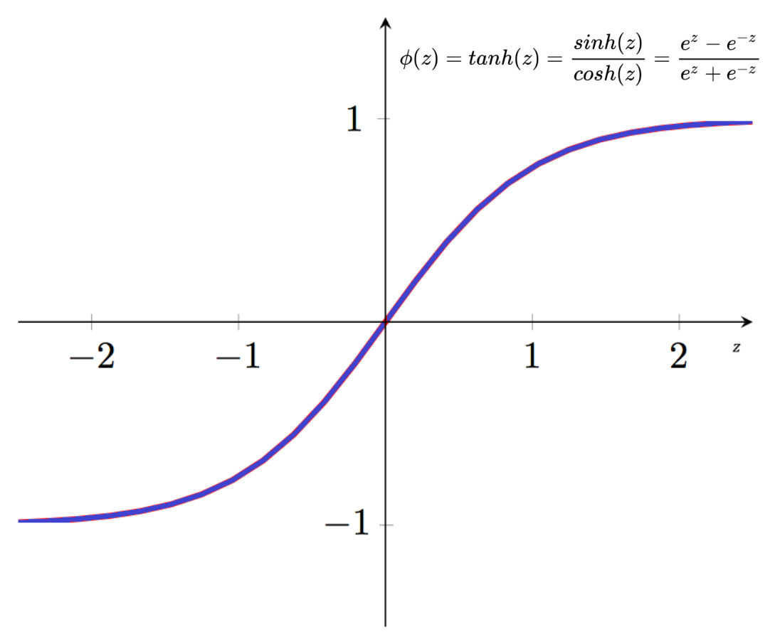
The hyperbolic tangent function is similar in appearance to the sigmoid function, but its output values are all shifted downwards.

How Do Neural Networks Really Work?

So far in this tutorial, we have discussed two of the building blocks for building neural networks:

• Neurons
• Activation functions

However, you’re probably still a bit confused as to how neural networks really work.

This tutorial will put together the pieces we’ve already discussed so that you can understand how neural networks work in practice.

The Example We’ll Be Using In This Tutorial

This tutorial will work through a real-world example step-by-step so that you can understand how neural networks make predictions.

More specifically, we will be dealing with property valuations.

You probably already know that there are a ton of factors that influence house prices, including the economy, interest rates, its number of bedrooms/bathrooms, and its location.

The high dimensionality of this data set makes it an interesting candidate for building and training a neural network on.

One caveat about this section is the neural network we will be using to make predictions has already been trained. We’ll explore the process for training a new neural network in the next section of this tutorial.

The Parameters In Our Data Set

Let’s start by discussing the parameters in our data set. More specifically, let’s imagine that the data set contains the following parameters:

• Square footage
• Bedrooms
• Distance to city center
• House age

These four parameters will form the input layer of the artificial neural network. Note that in reality, there are likely many more parameters that you could use to train a neural network to predict housing prices. We have constrained this number to four to keep the example reasonably simple.

The Most Basic Form of a Neural Network

In its most basic form, a neural network only has two layers – the input layer and the output layer. The output layer is the component of the neural net that actually makes predictions.

For example, if you wanted to make predictions using a simple weighted sum (also called linear regression) model, your neural network would take the following form:

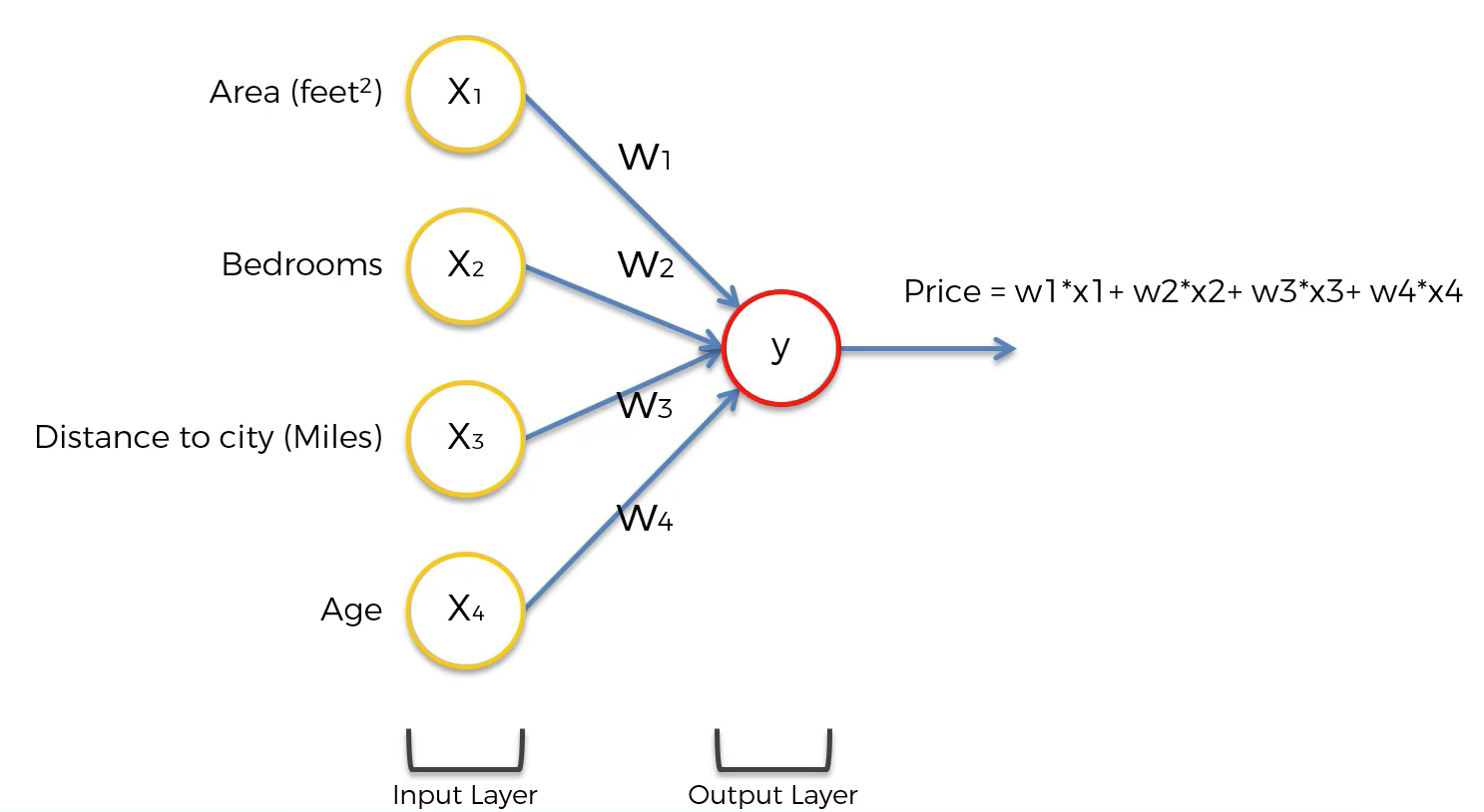
While this diagram is a bit abstract, the point is that most neural networks can be visualized in this manner:

• An input layer
• Possibly some hidden layers
• An output layer

It is the hidden layer of neurons that causes neural networks to be so powerful for calculating predictions.

For each neuron in a hidden layer, it performs calculations using some (or all) of the neurons in the last layer of the neural network. These values are then used in the next layer of the neural network.

The Purpose of Neurons in the Hidden Layer of a Neural Network

You are probably wondering – what exactly does each neuron in the hidden layer mean? Said differently, how should machine learning practitioners interpret these values?

Generally speaking, neurons in the midden layers of a neural net are activated (meaning their activation function returns 1) for an input value that satisfies certain sub-properties.

For our housing price prediction model, one example might be 5-bedroom houses with small distances to the city center.

In most other cases, describing the characteristics that would cause a neuron in a hidden layer to activate is not so easy.

How Neurons Determine Their Input Values

Earlier in this tutorial, I wrote “For each neuron in a hidden layer, it performs calculations using some (or all) of the neurons in the last layer of the neural network.”

This illustrates an important point – that each neuron in a neural net does not need to use every neuron in the preceding layer.

The process through which neurons determine which input values to use from the preceding layer of the neural net is called training the model. We will learn more about training neural nets in the next section of this course.

Visualizing A Neural Net’s Prediction Process

When visualizing a neutral network, we generally draw lines from the previous layer to the current layer whenever the preceding neuron has a weight above 0 in the weighted sum formula for the current neuron.

The following image will help visualize this:

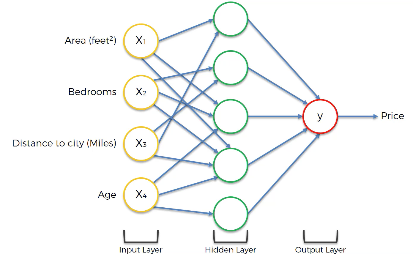
As you can see, not every neuron-neuron pair has synapse. x4 only feeds three out of the five neurons in the hidden layer, as an example. This illustrates an important point when building neural networks – that not every neuron in a preceding layer must be used in the next layer of a neural network.

How Neural Networks Are Trained

So far you have learned the following about neural networks:

• That they are composed of neurons
• That each neuron uses an activation function applied to the weighted sum of the outputs from the preceding layer of the neural network
• A broad, no-code overview of how neural networks make predictions

We have not yet covered a very important part of the neural network engineering process: how neural networks are trained.

Now you will learn how neural networks are trained. We’ll discuss data sets, algorithms, and broad principles used in training modern neural networks that solve real-world problems.

Hard-Coding vs. Soft-Coding

There are two main ways that you can develop computer applications. Before digging in to how neural networks are trained, it’s important to make sure that you have an understanding of the difference between hard-coding and soft-coding computer programs.

Hard-coding means that you explicitly specify input variables and your desired output variables. Said differently, hard-coding leaves no room for the computer to interpret the problem that you’re trying to solve.

Soft-coding is the complete opposite. It leaves room for the program to understand what is happening in the data set. Soft-coding allows the computer to develop its own problem-solving approaches.

A specific example is helpful here. Here are two instances of how you might identify cats within a data set using soft-coding and hard-coding techniques.

• Hard-coding: you use specific parameters to predict whether an animal is a cat. More specifically, you might say that if an animal’s weight and length lie within certain
• Soft-coding: you provide a data set that contains animals labelled with their species type and characteristics about those animals. Then you build a computer program to predict whether an animal is a cat or not based on the characteristics in the data set.

As you might imagine, training neural networks falls into the category of soft-coding. Keep this in mind as you proceed through this course.

Training A Neural Network Using A Cost Function

Neural networks are trained using a cost function, which is an equation used to measure the error contained in a network’s prediction.

The formula for a deep learning cost function (of which there are many – this is just one example) is below:

Note: this cost function is called the mean squared error, which is why there is an MSE on the left side of the equal sign.

While there is plenty of formula mathematics in this equation, it is best summarized as follows:

Take the difference between the predicted output value of an observation and the actual output value of that observation. Square that difference and divide it by 2.

To reiterate, note that this is simply one example of a cost function that could be used in machine learning (although it is admittedly the most popular choice). The choice of which cost function to use is a complex and interesting topic on its own, and outside the scope of this tutorial.

As mentioned, the goal of an artificial neural network is to minimize the value of the cost function. The cost function is minimized when your algorithm’s predicted value is as close to the actual value as possible. Said differently, the goal of a neural network is to minimize the error it makes in its predictions!

Modifying A Neural Network

After an initial neural network is created and its cost function is imputed, changes are made to the neural network to see if they reduce the value of the cost function.

More specifically, the actual component of the neural network that is modified is the weights of each neuron at its synapse that communicate to the next layer of the network.

The mechanism through which the weights are modified to move the neural network to weights with less error is called gradient descent. For now, it’s enough for you to understand that the process of training neural networks looks like this:

• Initial weights for the input values of each neuron are assigned
• Predictions are calculated using these initial values
• The predictions are fed into a cost function to measure the error of the neural network
• A gradient descent algorithm changes the weights for each neuron’s input values
• This process is continued until the weights stop changing (or until the amount of their change at each iteration falls below a specified threshold)

This may seem very abstract – and that’s OK! These concepts are usually only fully understood when you begin training your first machine learning models.

Final Thoughts

In this tutorial, you learned about how neural networks perform computations to make useful predictions.

If you’re interested in learning more about building, training, and deploying cutting-edge machine learning model, my eBook Pragmatic Machine Learning will teach you how to build 9 different machine learning models using real-world projects.

You can deploy the code from the eBook to your GitHub or personal portfolio to show to prospective employers. The book launches on August 3rd – preorder it for 50% off now!