Common architectures in convolutional neural networks.

In this post, I’ll discuss commonly used architectures for convolutional networks. As you’ll see, almost all CNN architectures follow the same general design principles of successively applying convolutional layers to the input, periodically downsampling the spatial dimensions while increasing the number of feature maps.

While the classic network architectures were comprised simply of stacked convolutional layers, modern architectures explore new and innovative ways for constructing convolutional layers in a way which allows for more efficient learning. Almost all of these architectures are based on a repeatable unit which is used throughout the network.

These architectures serve as general design guidelines which machine learning practitioners will then adapt to solve various computer vision tasks. These architectures serve as rich feature extractors which can be used for image classification, object detection, image segmentation, and many other more advanced tasks.

Classic network architectures (included for historical purposes)

Modern network architectures

LeNet-5

Yann Lecun’s LeNet-5 model was developed in 1998 to identify handwritten digits for zip code recognition in the postal service. This pioneering model largely introduced the convolutional neural network as we know it today.

Architecture

Convolutional layers use a subset of the previous layer’s channels for each filter to reduce computation and force a break of symmetry in the network. The subsampling layers use a form of average pooling.

Parameters: 60,000

Paper: Gradient-based learning applied to document recognition

AlexNet

AlexNet was developed by Alex Krizhevsky et al. in 2012 to compete in the ImageNet competition. The general architecture is quite similar to LeNet-5, although this model is considerably larger. The success of this model (which took first place in the 2012 ImageNet competition) convinced a lot of the computer vision community to take a serious look at deep learning for computer vision tasks.

Architecture

Parameters: 60 million

Paper: ImageNet Classification with Deep Convolutional Neural Networks

VGG-16

The VGG network, introduced in 2014, offers a deeper yet simpler variant of the convolutional structures discussed above. At the time of its introduction, this model was considered to be very deep.

Architecture

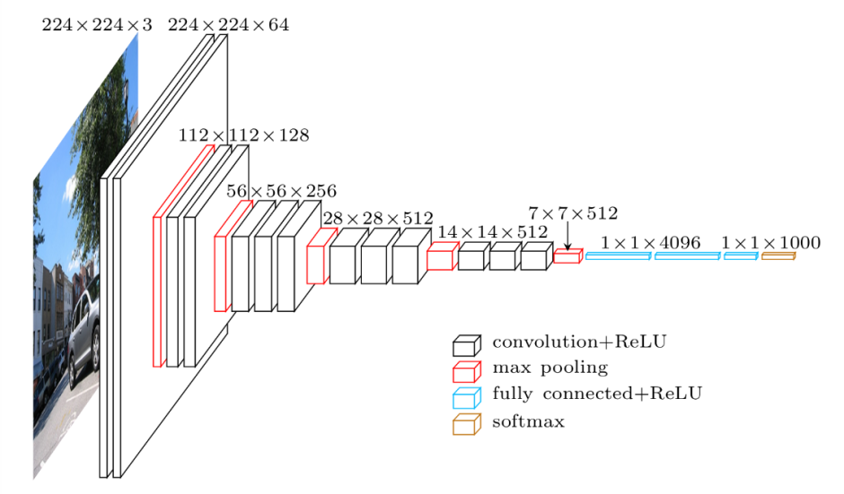
Parameters: 138 million

Paper: Very Deep Convolutional Networks for Large-Scale Image Recognition

Inception (GoogLeNet)

In 2014, researchers at Google introduced the Inception network which took first place in the 2014 ImageNet competition for classification and detection challenges.

The model is comprised of a basic unit referred to as an “Inception cell” in which we perform a series of convolutions at different scales and subsequently aggregate the results. In order to save computation, 1×1 convolutions are used to reduce the input channel depth. For each cell, we learn a set of 1×1, 3×3, and 5×5 filters which can learn to extract features at different scales from the input. Max pooling is also used, albeit with “same” padding to preserve the dimensions so that the output can be properly concatenated.

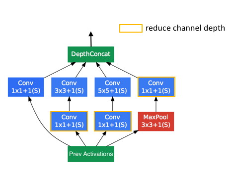
These researchers published a follow-up paper which introduced more efficient alternatives to the original Inception cell. Convolutions with large spatial filters (such as 5×5 or 7×7) are beneficial in terms of their expressiveness and ability to extract features at a larger scale, but the computation is disproportionately expensive. The researchers pointed out that a 5×5 convolution can be more cheaply represented by two stacked 3×3 filters.

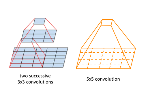
Whereas a $5 \times 5 \times c$ filter requires $25c$ parameters, two $3 \times 3 \times c$ filters only require $18c$ parameters. In order to most accurately represent a 5×5 filter, we shouldn’t use any nonlinear activations between the two 3×3 layers. However, it was discovered that “linear activation was always inferior to using rectified linear units in all stages of the factorization.”

It was also shown that 3×3 convolutions could be further deconstructed into successive 3×1 and 1×3 convolutions.

Generalizing this insight, we can more efficiently compute an $n \times n$ convolution as a $1 \times n$ convolution followed by a $n \times 1$ convolution.

Architecture

In order to improve overall network performance, two auxiliary outputs are added throughout the network. It was later discovered that the earliest auxiliary output had no discernible effect on the final quality of the network. The addition of auxiliary outputs primarily benefited the end performance of the model, converging at a slightly better value than the same network architecture without an auxiliary branch. It is believed the addition of auxiliary outputs had a regularizing effect on the network.

A revised, deeper version of the Inception network which takes advantage of the more efficient Inception cells is shown below.

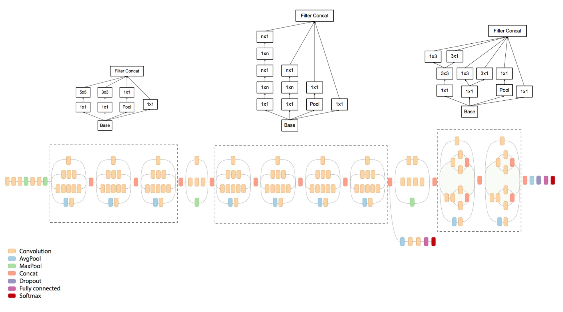
Parameters: 5 million (V1) and 23 million (V3)

Papers:

ResNet

Deep residual networks were a breakthrough idea which enabled the development of much deeper networks (hundreds of layers as opposed to tens of layers).

Its a generally accepted principle that deeper networks are capable of learning more complex functions and representations of the input which should lead to better performance. However, many researchers observed that adding more layers eventually had a negative effect on the final performance. This behavior was not intuitively expected, as explained by the authors below.

Let us consider a shallower architecture and its deeper counterpart that adds more layers onto it. There exists a solution by construction to the deeper model: the added layers are identity mapping, and the other layers are copied from the learned shallower model. The existence of this constructed solution indicates that a deeper model should produce no higher training error than its shallower counterpart. But experiments show that our current solvers on hand are unable to find solutions that are comparably good or better than the constructed solution (or unable to do so in feasible time).

This phenomenon is referred to by the authors as the degradation problem – alluding to the fact that although better parameter initialization techniques and batch normalization allow for deeper networks to converge, they often converge at a higher error rate than their shallower counterparts. In the limit, simply stacking more layers degrades the model’s ultimate performance.

The authors propose a remedy to this degradation problem by introducing residual blocks in which intermediate layers of a block learn a residual function with reference to the block input. You can think of this residual function as a refinement step in which we learn how to adjust the input feature map for higher quality features. This compares with a “plain” network in which each layer is expected to learn new and distinct feature maps. In the event that no refinement is needed, the intermediate layers can learn to gradually adjust their weights toward zero such that the residual block represents an identity function.

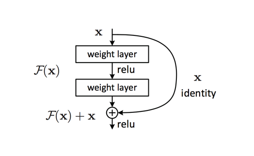
Note: It was later discovered that a slight modification to the original proposed unit offers better performance by more efficiently allowing gradients to propagate through the network during training.

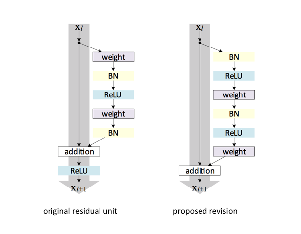
Wide residual networks
Although the original ResNet paper focused on creating a network architecture to enable deeper structures by alleviating the degradation problem, other researchers have since pointed out that increasing the network’s width (channel depth) can be a more efficient way of expanding the overall capacity of the network.

Architecture

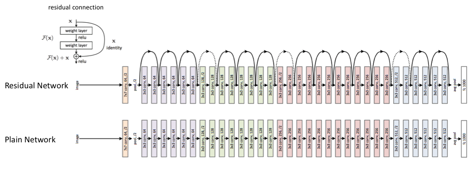
Each colored block of layers represent a series of convolutions of the same dimension. The feature mapping is periodically downsampled by strided convolution accompanied by an increase in channel depth to preserve the time complexity per layer. Dotted lines denote residual connections in which we project the input via a 1×1 convolution to match the dimensions of the new block.

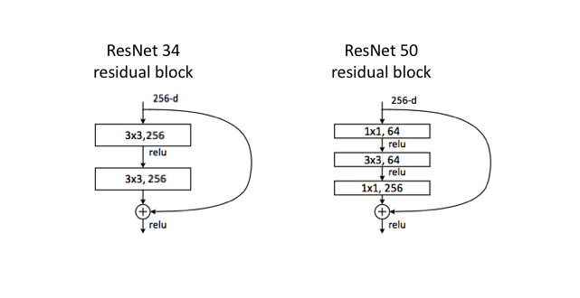
The diagram above visualizes the ResNet 34 architecture. For the ResNet 50 model, we simply replace each two layer residual block with a three layer bottleneck block which uses 1×1 convolutions to reduce and subsequently restore the channel depth, allowing for a reduced computational load when calculating the 3×3 convolution.

Parameters: 25 million (ResNet 50)

Papers:

ResNeXt

The ResNeXt architecture is an extension of the deep residual network which replaces the standard residual block with one that leverages a “split-transform-merge” strategy (ie. branched paths within a cell) used in the Inception models. Simply, rather than performing convolutions over the full input feature map, the block’s input is projected into a series of lower (channel) dimensional representations of which we separately apply a few convolutional filters before merging the results.

This idea is quite similar to group convolutions, which was an idea proposed in the AlexNet paper as a way to share the convolution computation across two GPUs. Rather than creating filters with the full channel depth of the input, the input is split channel-wise into groups with each as shown below.

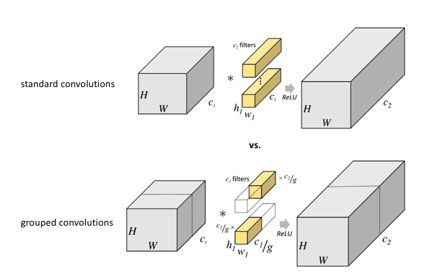
It was discovered that using grouped convolutions led to a degree of specialization among groups where separate groups focused on different characteristics of the input image.

The ResNeXt paper refers to the number of branches or groups as the cardinality of the ResNeXt cell and performs a series of experiments to understand relative performance gains between increasing the cardinality, depth, and width of the network. The experiments show that increasing cardinality is more effective at benefiting model performance than increasing the width or depth of the network. The experiments also suggest that “residual connections are helpful for optimization, whereas aggregated transformations are (helpful for) stronger representations.”

Architecture

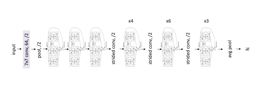
The ResNeXt architecture simply mimicks the ResNet models, replacing the ResNet blocks for the ResNeXt block.

Paper: Aggregated Residual Transformations for Deep Neural Networks

DenseNet

The idea behind dense convolutional networks is simple: it may be useful to reference feature maps from earlier in the network. Thus, each layer’s feature map is concatenated to the input of every successive layer within a dense block. This allows later layers within the network to directly leverage the features from earlier layers, encouraging feature reuse within the network. The authors state, “concatenating feature-maps learned by different layers increases variation in the input of subsequent layers and improves efficiency.”

When I first came across this model, I figured that it would have an absurd number of parameters to support the dense connections between layers. However, because the network is capable of directly using any previous feature map, the authors found that they could work with very small output channel depths (ie. 12 filters per layer), vastly reducing the total number of parameters needed. The authors refer to the number of filters used in each convolutional layer as a “growth rate”, $k$, since each successive layer will have $k$ more channels than the last (as a result of accumulating and concatenating all previous layers to the input).

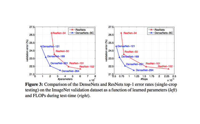
When compared with ResNet models, DenseNets are reported to acheive better performance with less complexity.

Architecture

For a majority of the experiments in the paper, the authors mimicked the general ResNet model architecture, simply swapping in the dense block as the repeated unit.

Parameters:

• 0.8 million (DenseNet-100, k=12)
• 15.3 million (DenseNet-250, k=24)
• 40 million (DenseNet-190, k=40)

Paper: Densely Connected Convolutional Networks
Video: CVPR 2017 Best Paper Award: Densely Connected Convolutional Networks

Further reading

An Analysis of Deep Neural Network Models for Practical Applications
– Corresponding blog post