Introduction

Tutorial Dependencies

Before you start this tutorial, you should probably be familiar with basic python. There are also some basic concepts of linear algebra and calculus involved. If you aren’t there yet, it’s all good! We’re going to do our best to explain it as we go!

Before we get started with the how of building a Neural Network, we need to understand the what first.

Neural networks can be intimidating, especially for people new to machine learning. However, this tutorial will break down how exactly a neural network works and you will have a working flexible neural network by the end. Let’s get started!

Understanding the Process

With approximately 100 billion neurons, the human brain processes data at speeds as fast as 268 mph! In essence, a neural network is a collection of neurons connected by synapses. This collection is organized into three main layers: the input layer, the hidden layer, and the output layer. You can have many hidden layers, which is where the term deep learning comes into play. In an artificial neural network, there are several inputs, which are called features, and a single output is produced, which is called a label.

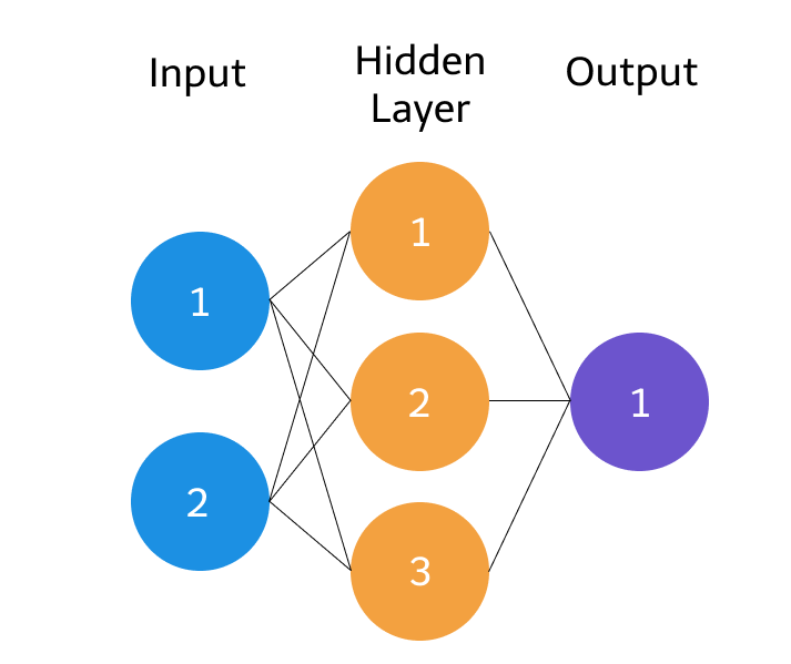
The circles represent neurons while the lines represent synapses. The role of a synapse is to multiply the inputs and weights. You can think of weights as the “strength” of the connection between neurons. Weights primarily define the output of a neural network. However, they are highly flexible. After, an activation function is applied to return an output.

Here’s a brief overview of how a simple feedforward neural network works. We’ll be going through the following steps in the tutorial. Don’t worry if some of these terms feel unfamiliar.

1. Takes inputs as a matrix (2D array of numbers)
2. Multiplies the input by a set of weights
3. Applies an activation function
4. Returns an output (a prediction)
5. Error is calculated by taking the difference from the desired output from the data and the predicted output. This creates our gradient descent, which we can use to alter the weights.
6. The weights are then altered slightly according to the error.
7. To train, this process is repeated 1,000+ times. The more the data is trained upon, the more accurate our outputs will be.

At its core, neural networks are simple. They perform a dot product with the input and weights and apply an activation function. When weights are adjusted via the gradient of loss function, the network adapts to the changes to produce more accurate outputs.

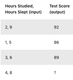
Our neural network will model a single hidden layer with three inputs and one output. In the network, we will be predicting the score of our exam based on the inputs of how many hours we studied and how many hours we slept the day before. Our test score is the output. Here’s our sample data of what we’ll be training our neural network on:

Setting Up

Files & Libraries

This setup is pretty simple! Just create a main.py file in your favorite IDE! Before we start coding, we’ll want to have Numpy installed. Why are we using Numpy? Numpy is a really powerful library that allows us to do cool stuff with matrices. Some things to know about how they’re different from Python lists:

1. Numpy arrays are homogeneous (they all have the same data type inside them)
2. Because they are homogenous, they can perform computations orders of magnitudes faster
3. Numpy is most often used in scientific computing and research

If don’t have Numpy, you can install it with this command:

pip install numpy

If you’re running Anaconda, type this in your conda environment (if you’re not, just move on!)

conda activate  
conda install numpy

We’ll start with importing numpy in main.py.

import
 numpy 
as
 np

Exercise: Normalization of Training Data

To get started, we’ll need to load in our training data.

First, let’s import our training input data of hours studied and hours slept as numpy arrays using np.array.

 
x_all = np.array(([
2
, 
9
], [
1
, 
5
], [
3
, 
6
], [
5
, 
10
]), dtype=float)  

Based on the example above, set y equal to a np.array with our training output data of test scores as well.

Solution

y = np.array(([
92
], [
86
], [
89
]), dtype=float)  

Scaling our training data

Next, we’ll want to scale our training input data to make sure that all our datapoints are between 0 and 1. To do this, we will scale our units by dividing each element by the maximum value in the array. Why scale the data? This allows us to see all of the data in proportion to itself. Feature normalization like this is an important part of preprocessing when training machine learning models.

 
x_all = x_all/np.max(x_all, axis=
0
)  

Now try scaling the y data! Think about what the maximum test score is.

Solution

y = y/
100
  

Splitting our training data

We need to split our data into training and testing data. We want to have data to test our neural network on, so let’s use some of what we have. Here we are splitting the training data at index 3. The split function gives us an array where the first value is the list of everything before the index, and the second value is the list of everything at the index and after. Here is how we would split the training data.

 
X = np.split(x_all, [
3
])[
0
]  

Now try setting the testing data to x_predicted.

Solution

x_predicted = np.split(x_all, [
3
])[
1
]  

Feel free to print these arrays using print(str(X)) to see what the data looks like.

Summary of Your Progress

Here is what our file should look like so far!

 
x_all = np.array(([
2
, 
9
], [
1
, 
5
], [
3
, 
6
], [
5
, 
10
]), dtype=float)  
y = np.array(([
92
], [
86
], [
89
]), dtype=float)  

 
x_all = x_all/np.max(x_all, axis=
0
)  
y = y/
100
  

 
X = np.split(x_all, [
3
])[
0
]  
x_predicted = np.split(x_all, [
3
])[
1
]  

To summarize, we imported, normalized, and split our training data. The data is imported into the arrays x_all and y and then scaled. We did this by dividing each point by the maximum point in each array. For example, for our x_all array, 2, 1, and 3 was divided by 5 , then 9, 5, and 6 was divided by 10. We did the same for our y output array. Then, we split our input data into training and testing data. The first three data points are what we will train the network on. Then, we will ask the network to predict the test score for someone who studies for 5 hours and sleeps for 10 hours as evident in the x_predicted array.

Forward Propagation

What is Forward Propagation?

So far we have the data all set up. Now let’s see if we can predict a score for our input data.

Forward propagation is how our neural network predicts a score for input data.

Here’s how the first input data element (2 hours studying and 9 hours sleeping) would calculate an output in the network:

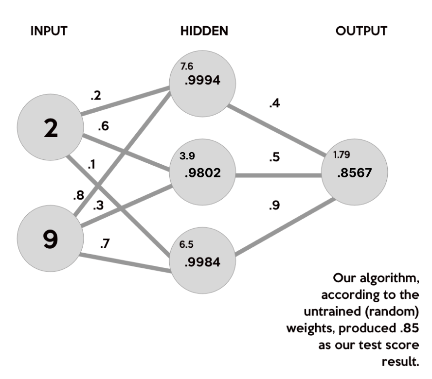
Don’t worry about all the numbers just yet! We will go through what this diagram means very soon. This is just to give you a taste for what you will be calculating. Our neural network will have two neurons in the input layer, three neurons in the hidden layer and 1 neuron for the output layer.

Creating a Neural Network Class

Next, let’s define a python class and write an init function where we’ll specify our parameters such as the input, hidden, and output layers.

class
 
neural_network
(object)
:  
    
def
 
__init__
(self)
:
     
        self.inputSize = 
2
    
        self.outputSize = 
1
    
        self.hiddenSize = 
3

Calculations Behind Our Network

It is time for our first calculation.

Here is that diagram again!

Let’s break it down. Our neural network can be represented with matrices. We take the dot product of each row of the first matrix and each column of the second matrix. What’s the dot product? The dot product is the sum of the products of the elements. This is done element-wise. So, in order to get the first element in the hidden layer matrix, you multiply 2 by .2 and add that to 9 times .8 to get 7.6.

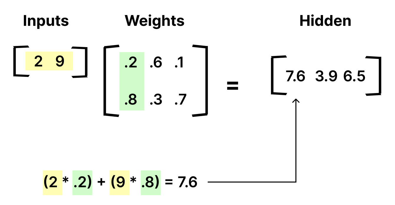
Once you repeat this process for all the columns in the weights matrix, you get all the hidden layer neuron values which are shown in the hidden layer matrix on the right.

(
2
 * 
.2
) + (
9
 * 
.8
) = 
7.6
(
2
 * 
.6
) + (
9
 * 
.3
) = 
3.9
(
2
 * 
.1
) + (
9
 * 
.7
) = 
6.5

This is the fundamental concept behind forward propagation. Now, let’s put all the other inputs into the inputs matrix.

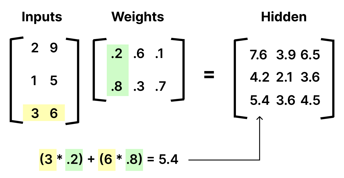
As you might notice, every time we move down a row in the inputs, we move down a row in the result. This is a lot to digest, so take a moment to ponder what is happening here.

The full matrices are a lot of numbers to think about. When you consider what happens in the network, first think about what happens with only one row of the inputs before generalizing to all of them.

Now that we understand the math, let’s remind ourselves of the diagram showing forward propagation for just the first row of the input layer.

The values we got in our hidden matrix are in the small font on the top left, why? Well, we must apply the activation function on each of these values. In an artificial neural network, an activation function of a neuron defines the output of the neuron given a set of inputs. In other words, activation functions give a network a sense of how activated a neuron is by mapping the input set to some value in between a given lower and upper bound. This is inspired by biology as certain Neural_Networkneurons within our brains are either firing or not depending on stimuli. You may think of a neuron firing as represented with a 1 and a neuron not firing as represented with a 0.

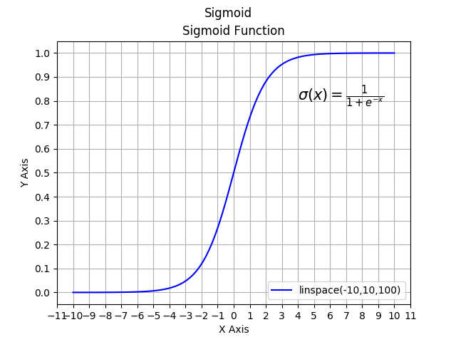
There are many activation functions out there. In this case, we’ll stick to one of the more popular ones — the sigmoid function. The sigmoid function maps all input values to some value between a lower limit of 0 and an upper limit of 1. If the input is very negative, the number will be transformed into a number very close to 0. If the input is very positive, the number will be transformed to a number very close to 1. If the input is close to 0, the number will be transformed into some number in between 0 and 1.

S(
7.6
) = 
0.9994997
S(
3.9
) = 
0.9801597
S(
6.5
) = 
0.9984988

Now, we need to use matrix multiplication again, with another set of random weights, to calculate our output layer value.

(
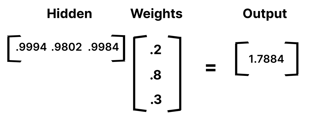
.9994
 * 
.4
) + (
.9802
 * 
.5
) + (
.9984
 * 
.9
) = 
1.78842

Lastly, to normalize the output, we just apply the activation function again.

S(
1.78842
) = 
.8567335

And, there you go! We just did forward propagation! With those weights, our neural network will calculate .85 as our test score! However, our target was .92. Our result wasn’t poor, it just isn’t the best it can be. We just got a little lucky when we chose the random weights for this example.

How do we train our model to learn? Well, we’ll find out very soon. For now, let’s continue coding our network.

If you are still confused, I highly recommend you check out this informative video which explains the structure of a neural network with the same example.

Implementing the calculations

Now, let’s generate our weights randomly using np.random.randn(). Remember, we’ll need two sets of weights because we are building two layers: the hidden layer and the output layer. One set of weights goes from the input to the hidden layer, and the other goes from the hidden to output layer.

 
self.W1 = np.random.randn(self.inputSize, self.hiddenSize)  
self.W2 = np.random.randn(self.hiddenSize, self.outputSize)  

Once we have all the variables set up, we are ready to write our forward propagation function. Let’s pass in our input, X, and in this example, we can use the variable z to simulate the activity between the input and output layers. As explained, we need to take a dot product of the inputs and weights, apply an activation function, take another dot product of the hidden layer and second set of weights, and lastly apply a final activation function to receive our output:

The last thing we need before we create our forward propagation function is to define our sigmoid function, which is our activation function that we learned about before:

def
 
sigmoid
(self, s)
:
   
  
return
 
1
/(
1
+np.exp(-s))

This is simply the equation for the sigmoid function, a type of a logistic function, and it looks like this:

Now onto the forward function

For this function, we want to define the forward propagation through our neural network. First, we take the dot product of our input with the first set of random weights. Now, it’s ready to be activated! We will apply the sigmoid function element-wise to the matrix. Using Numpy is really nice for this because we can just call the sigmoid function we just defined to be applied on the entire matrix we just computed by taking the dot product of our input with the first set of weights. See the beginning of our forward function below.

def
 
forward
(self, X)
:
 
  self.z = np.dot(X, self.W1)  
  self.z2 = self.sigmoid(self.z)  

Exercise: Building a Layer

Now it’s your turn. Define the next layer of the neural network by dotting the second set of hidden weights with z2 and call this variable z3. Then apply the activation function to it. Since this is our output, don’t forget to return it!

Solution

def
 
forward
(self, X)
:
 

  self.z = np.dot(X, self.W1)  
  self.z2 = self.sigmoid(self.z)  

   
  self.z3 = np.dot(self.z2, self.W2)  
  o = self.sigmoid(self.z3)  
  
return
 o

As you can see in the code, we just did the same thing for the second layer of the network. Using the activated z2 layer, we took the dot product with the next set of random weights and then applied the activation function to it. Because it was the last layer of the network, we return the results by typing return o.

Finally, let’s define our neural network class and get our predicted and actual outputs using the data we have

nn = neural_network()

 
o = nn.forward(X)

print
 
"Predicted Output: \n"
 + str(o)
print
 
"Actual Output: \n"
 + str(y)

Summary of Your Progress

And there we have it! In this module, we learned about forward propagation and our activation function. We created randomized weights and fed them forward through the network by means of the dot product and activation function. Finally, we made our first predictions!

Full Code

import
 numpy 
as
 np

 
x_all = np.array(([
2
, 
9
], [
1
, 
5
], [
3
, 
6
], [
5
, 
10
]), dtype=float)  
y = np.array(([
92
], [
86
], [
89
]), dtype=float)  

 
x_all = x_all/np.amax(x_all, axis=
0
)  
y = y/
100
  

 
X = np.split(x_all, [
3
])[
0
]  
x_predicted = np.split(x_all, [
3
])[
1
]  

class
 
neural_network
(object)
:
  
def
 
__init__
(self)
:
     
    self.inputSize = 
2
    self.outputSize = 
1
    self.hiddenSize = 
3

     
    self.W1 = np.random.randn(self.inputSize, self.hiddenSize)  
    self.W2 = np.random.randn(self.hiddenSize, self.outputSize)  

  
def
 
forward
(self, X)
:
     
    self.z = np.dot(X, self.W1)  
    self.z2 = self.sigmoid(self.z)  
    self.z3 = np.dot(self.z2, self.W2)  
    o = self.sigmoid(self.z3)  
    
return
 o

  
def
 
sigmoid
(self, s)
:
     
    
return
 
1
/(
1
+np.exp(-s))

nn = neural_network()

 
o = nn.forward(X)

print
 
"Predicted Output: \n"
 + str(o)
print
 
"Actual Output: \n"
 + str(y)

As you may have noticed, we need to train our network to calculate more accurate results.

Backpropagation

The “Learning” of Our Network

Since we have a random set of weights, we need to alter them to make our neural network guess the correct test scores. This is done through a method called backpropagation.

Backpropagation works by using a loss function to calculate how far the network was from the target output.

What does backpropagation adjust to make the neural network better at guessing the correct values?

A) Loss values

B) Gradient descent

C) Activation function

D) Weights

Solution

D) Weights

Calculating Error

One way of representing the loss (cost) function is by using the mean squared error function:

In this function, o is our predicted output, and y is our actual output. The mean squared error function is the sum, over all the data points, of the square of the difference between the predicted and actual target variables, divided by the number of data points. We’ll get into coding this soon.

Bias in Neural Networks

In a neural network, we would ideally would want to have a bias. A bias allows us to shift the activation function either to the right or left, which means that we would be able to fit the prediction with the input data much better. The initial bias is dependent on your dataset, but this value should be updated along with the weights during backpropagation.

For the sake of simplicity, we assume bias to be 0 in this tutorial.

Gradient Descent

Now that we have the loss (cost) function, our goal is to get it as close as we can to 0. As we are training our network, all we are doing is minimizing the loss function. In other words, we are optimizing to find the local minimum of our loss function.

If you remember, our loss function is dependent on our output, which is dependent on our weights. We could brute force search all possible combinations of weights to minimize loss. However, this would take a really, really, really long time and just isn’t practical. We need an intuitive method to find the local minimum of the loss function.

For this optimization, we will use the method of gradient descent. Let’s look at the function f(x), where x is our input weight and f(x) is our loss function. What if we could take the derivative at a given weight? This would allow us to understand which way is downhill and whether to make our x (weight) smaller or larger to decrease our loss. In other words, to figure out which direction to alter our weights, we need to find the rate of change of our loss with respect to our weights (a partial derivative!).

If this partial derivative of our loss with respect to our weights is positive, then the cost function is going uphill. If it is negative, then the cost function is going downhill. Therefore, we’re able to save time by making sure that we’re optimizing in the right direction.

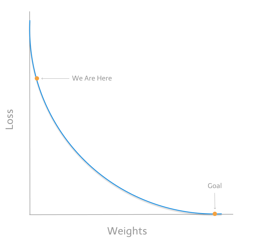
Above is an illustration describing our method of gradient descent. By knowing which way to alter our weights, our outputs can only get more accurate.

Here’s how we will calculate the incremental change to our weights:

1. Find the margin of error of the output layer (o) by taking the difference of the predicted output and the actual output (y)
2. Apply the derivative of our sigmoid activation function to the output layer error. We call this result the delta output sum.
3. Use the delta output sum of the output layer error to figure out how much our z2 (hidden) layer contributed to the output error by performing a dot product with our second weight matrix. We can call this the z2 error.
4. Calculate the delta output sum for the z2 layer by applying the derivative of our sigmoid activation function (just like step 2).
5. Adjust the weights for the first layer by performing a dot product of the input layer with the hidden (z2) delta output sum. For the second layer, perform a dot product of the hidden(z2) layer and the output (o) delta output sum.

Calculating the delta output sum and then applying the derivative of the sigmoid function are very important to backpropagation. The derivative of the sigmoid, also known as sigmoid prime, will give us the rate of change, or slope, of the activation function at the output sum.

Let’s continue to code our neural_network class by adding a sigmoidPrime (derivative of sigmoid) function:

def
 
sigmoidPrime
(self, s)
:   
    
return
 s * (
1
 - s)

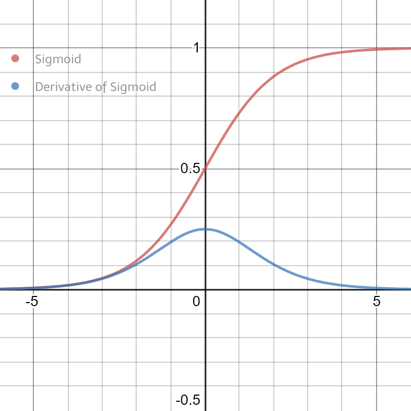
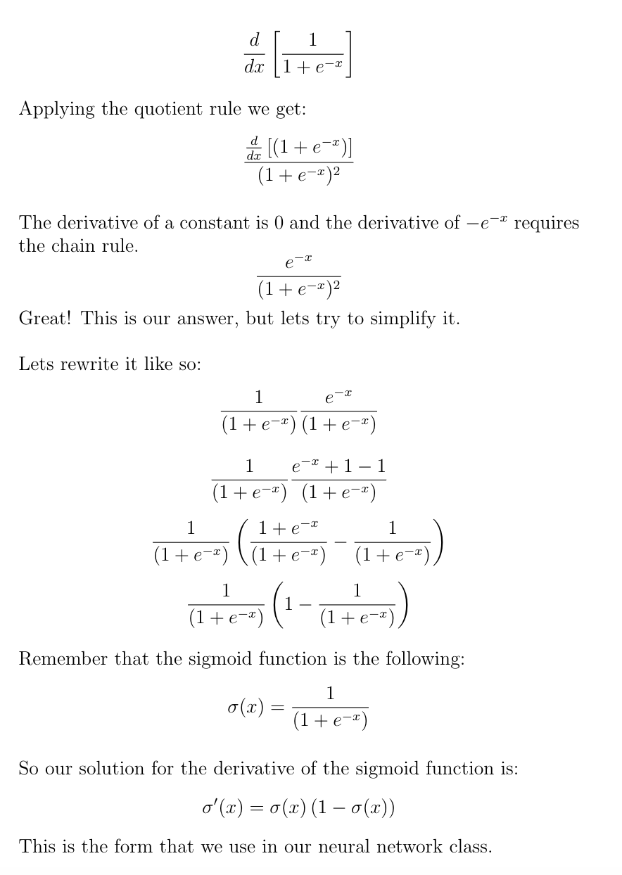
Here is an illustration of what the derivative of the sigmoid function looks like. The value is very small when you get far from 0 and gets larger only close to 0. Basically, when the neural network is very sure about a certain neuron, we do not want to change the value of that neuron and passing the value of the neuron through the sigmoid derivative will help with that. On the other hand, if the neural network is not as sure about the neuron, we want to change it more. You can find a full derivation of the sigmoid function in the appendix of this project!

Putting it All Together

Let’s implement our backward propagation function by using the method of gradient descent we just discovered.

First, we will find the error in our function by taking the difference of our output layer (o) and the actual value (y). Next we need to figure out how much to change the output layer, so we calculate this delta by multiplying the error of the output layer with the derivative of the sigmoid function. Luckily, we’ve already defined a function for this.

Once we’ve figured out the delta output sum for o, we go back to the hidden layer, z2, and calculate its error by taking the dot product of our o_delta and the transpose of the weights we used on it, W2. The reason we use the transpose of the second set of weights is so that we can apply the error of the output to each weight. Remember that o and W2 are 3×1 matrices; in order to do multiplication via the dot product W2 is transposed so the resulting matrix for z2_error is 3×3.

Next, we do the same thing as we did with the output error and multiply the error by the derivative of the sigmoid function to figure out the change in z2.

Now, we adjust our weights accordingly. Let’s adjust the first set of weights by dotting our input with the change in the hidden layer. We take the transpose again to make the multiplication possible. Then we can combine the result with the first set of weights, element-wise (thanks Numpy!). We do the same thing to the second set of weights except we use the hidden layer and the output layer to do so.

def
 
backward
(self, X, y, o)
:   
    self.o_error = y - o  
    self.o_delta = self.o_error*self.sigmoidPrime(o)  
    self.z2_error = self.o_delta.dot(self.W2.T)  
    self.z2_delta = self.z2_error*self.sigmoidPrime(self.z2)  
    self.W1 += X.T.dot(self.z2_delta)  
    self.W2 += self.z2.T.dot(self.o_delta)  

We can now define our output through initiating foward propagation and intiate the backward function by calling it in the train function:

Exercise: Creating the train function

Let’s combine our knowledge of forward and back propagation now to train the neural network! Define a function with parameters of your input, X, and output, y, that uses the forward and back propagation functions. Here’s a hint: remember the initial output is the result of forward propagation and that it gets fed into the backward function with your original parameters.

Solution

def
 
train
 
(self, X, y)
:  
  o = self.forward(X)  
  self.backward(X, y, o)

To run the network, all we have to do is to run the train function. Of course, we’ll want to do this multiple, or maybe thousands, of times. So, we’ll use a for loop.

Exercise: Defining Loss

Here’s a quick one. We’ve already defined the for loop to run our neural network a thousand times. Fill in the calculation for the loss function below! Take the mean of the square of the difference between the predicted and the actual output.

nn = neural_network()
for
 i 
in
 range(
1000
):  
  print(
"Input: \n"
 + str(X))
  print(
"Actual Output: \n"
 + str(y))
  print(
"Predicted Output: \n"
 + str(nn.forward(X)))
  print(
"Loss: \n"
 + str(
"fill me in!"
))  
  print(
"\n"
)
  nn.train(X, y)

Solution

  print(
"Loss: \n"
 + str(np.mean(np.square(y - nn.forward(X)))))  

Why take the square? Some of the errors will be negative. So, if we averaged the errors without squaring we might get close to 0 when the real loss is much larger. This Loss value is simply a way to quantify how far we are from the ‘perfect’ neural network.

Summary of Your Progress

Great, we now have a neural network! We discussed how to calculate the loss function and learned about gradient descent. We applied these two concepts to go backwards through the network to adjust our weights in the optimal direction. To put it all together, we trained our network to predict test scores using forward propagation, then backwards to perfect the weights we used.

What about using these trained weights to predict test scores that we don’t know?

Predictions

Exercise: Predict Function

Now, let’s create a new function that prints our predicted output for x_predicted. All we have to run is forward(x_predicted) to return an output!

Let’s write a predict member function within our class that prints out the input x_predicted matrix and the output matrix after it is passed into the forward() function.

Solution

def
 
predict
(self)
:
  print(
"Predicted data based on trained weights: "
)
  print(
"Input (scaled): \n"
 + str(x_predicted))
  print(
"Output: \n"
 + str(self.forward(x_predicted)))

To run this function simply call it under the for loop.

nn.predict()

If you’d like to save your trained weights, you can do so with np.savetxt:

def
 
saveWeights
(self)
:
  np.savetxt(
"w1.txt"
, self.W1, fmt=
"%s"
)
  np.savetxt(
"w2.txt"
, self.W2, fmt=
"%s"
)

Here’s the final program:

import
 numpy 
as
 np

 
x_all = np.array(([
2
, 
9
], [
1
, 
5
], [
3
, 
6
], [
5
, 
10
]), dtype=float)  
y = np.array(([
92
], [
86
], [
89
]), dtype=float)  

 
x_all = x_all/np.amax(x_all, axis=
0
)  
y = y/
100
  

 
X = np.split(x_all, [
3
])[
0
]  
x_predicted = np.split(x_all, [
3
])[
1
]  

class
 
neural_network
(object)
:
  
def
 
__init__
(self)
:
   
    self.inputSize = 
2
    self.outputSize = 
1
    self.hiddenSize = 
3

   
    self.W1 = np.random.randn(self.inputSize, self.hiddenSize)  
    self.W2 = np.random.randn(self.hiddenSize, self.outputSize)  

  
def
 
forward
(self, X)
:
     
    self.z = np.dot(X, self.W1)  
    self.z2 = self.sigmoid(self.z)  
    self.z3 = np.dot(self.z2, self.W2)  
    o = self.sigmoid(self.z3)  
    
return
 o

  
def
 
sigmoid
(self, s)
:
     
    
return
 
1
/(
1
+np.exp(-s))

  
def
 
sigmoidPrime
(self, s)
:
     
    
return
 s * (
1
 - s)

  
def
 
backward
(self, X, y, o)
:
     
    self.o_error = y - o  
    self.o_delta = self.o_error*self.sigmoidPrime(o)  

    self.z2_error = self.o_delta.dot(self.W2.T)  
    self.z2_delta = self.z2_error*self.sigmoidPrime(self.z2)  

    self.W1 += X.T.dot(self.z2_delta)  
    self.W2 += self.z2.T.dot(self.o_delta)  

  
def
 
train
(self, X, y)
:
    o = self.forward(X)
    self.backward(X, y, o)

  
def
 
saveWeights
(self)
:
    np.savetxt(
"w1.txt"
, self.W1, fmt=
"%s"
)
    np.savetxt(
"w2.txt"
, self.W2, fmt=
"%s"
)

  
def
 
predict
(self)
:
    print(
"Predicted data based on trained weights: "
)
    print(
"Input (scaled): \n"
 + str(x_predicted))
    print(
"Output: \n"
 + str(self.forward(x_predicted)))

nn = neural_network()
for
 i 
in
 range(
1000
):  
  print(
"# "
 + str(i) + 
"\n"
)
  print(
"Input (scaled): \n"
 + str(X))
  print(
"Actual Output: \n"
 + str(y))
  print(
"Predicted Output: \n"
 + str(nn.forward(X)))
  print(
"Loss: \n"
 + str(np.mean(np.square(y - nn.forward(X)))))  
  print(
"\n"
)
  nn.train(X, y)

nn.saveWeights()
nn.predict()

Here’s what I got after training the network 150,000 times. Keep in mind that doing this is grossly overfitting our data: training to essentially memorize the testing set. Models like these aren’t very useful for making predictions on data that does not originate from the dataset.

 

Input (scaled):
[[
0.4
 
0.9
]
 [
0.2
 
0.5
]
 [
0.6
 
0.6
]]
Actual Output:
[[
0.92
]
 [
0.86
]
 [
0.89
]]
Predicted Output:
[[
0.92
]
 [
0.86
]
 [
0.89
]]
Loss:
5.904467817735647e-17

Predicted data based on trained weights:
Input (scaled):
[[
1.
 
1.
]]
Output:
[[
0.93545994
]]

Project Summary

There you have it! A full-fledged neural network that can learn and adapt to produce accurate outputs. While we thought of our inputs as hours studying and sleeping, and our outputs as test scores, feel free to change these to whatever you like and observe how the network adapts! After all, all the network sees are the numbers. The calculations we made, as complex as they seemed to be, all played a big role in our learning model. If you think about it, it’s super impressive that your computer, a physical object, managed to learn by itself!

Appendix

Derivation of Sigmoid Prime

Visualizing Cost Per Iteration

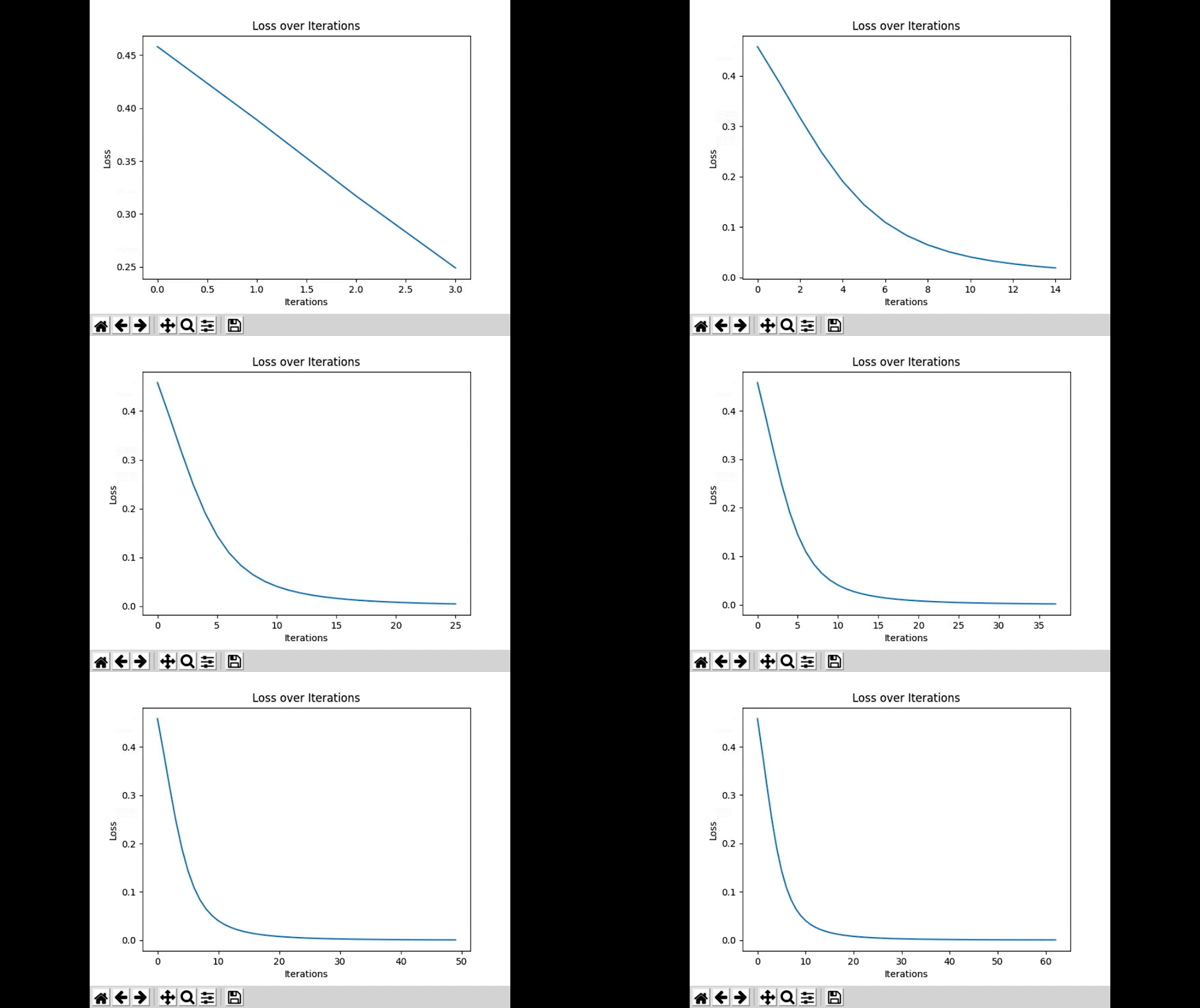
To plot our cost per iteration, we can use the matplotlib library. You can install and import the library like this:

pip install matplotlib  
conda install matplotlib  

import
 matplotlib.pyplot 
as
 plt

Let’s start be defining the count and loss lists to store iteration count and loss values respectively (we can do this above our for loop).

count = []  
loss = []  

Within our for loop, we can append our iteration into the count list and the loss output to the loss list. This can be plotted in real-time by first clearing the plot using plt.cla() and then calling the plt.plot(count, loss) function. We can also set a title using plt.title() and labels using plt.xlabel() , and plt.ylabel(). Lastly, we call plt.pause(.001) to specify how long the program should wait before plotting the data again.

for
 i 
in
 range(
1000
):  
  print(
"# "
 + str(i) + 
"\n"
)
  print(
"Input (scaled): \n"
 + str(X))
  print(
"Actual Output: \n"
 + str(y))
  print(
"Predicted Output: \n"
 + str(nn.forward(X)))
  loss = str(np.mean(np.square(y - nn.forward(X))))
  print(
"Loss: \n"
 +  loss )  
  print(
"\n"
)
  count.append(i)
  loss.append(np.round(float(loss), 
6
))
  plt.cla()
  plt.title(
"Loss over Iterations"
)
  plt.xlabel(
"Iterations"
)
  plt.ylabel(
"Loss"
)
  plt.plot(count, loss)
  plt.pause(
.001
)
  nn.train(X, y)

Awesome! You now have a real time graph for how your neural network learns. It feels like magic sometimes, but at the end of the day, any neural network is simply trying to get loss to 0.

Check it out here with these links!

Here’s the repl.it with the full code for real time graphing

Here’s the repl.it with the full code for the whole graph

References

Steven Miller

Welch Labs