Artificial Neural Network | Brilliant Math & Science Wiki

Neurons are connected to one another, with each neuron’s incoming connections made up of the outgoing connections of other neurons. Thus, the ANN will need to connect the outputs of sigmoidal units to the inputs of other sigmoidal units.

One Sigmoidal Unit

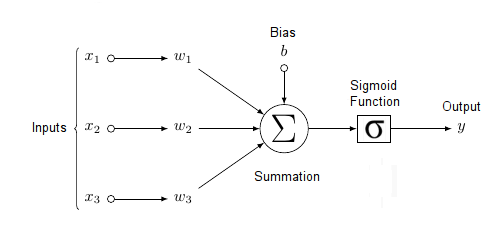
The diagram below shows a sigmoidal unit with three inputs \(\vec{x} = (x_1, x_2, x_3)\), one output \(y\), bias \(b\), and weight vector \(\vec{w} = (w_1, w_2, w_3)\). Each of the inputs \(\vec{x} = (x_1, x_2, x_3)\) can be the output of another sigmoidal unit (though it could also be raw input, analogous to unprocessed sense data in the brain, such as sound), and the unit’s output \(y\) can be the input to other sigmoidal units (though it could also be a final output, analogous to an action associated neuron in the brain, such as one that bends your left elbow). Notice that each component \(w_i\) of the weight vector corresponds to each component \(x_i\) of the input vector. Thus, the summation of the product of the individual \(w_i, x_i\) pairs is equivalent to the dot product, as discussed in the previous sections.

ANNs as Graphs

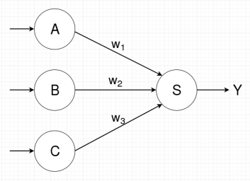
Artificial neural networks are most easily visualized in terms of a directed graph. In the case of sigmoidal units, node \(s\) represents sigmoidal unit \(s\) (as in the diagram above) and directed edge \(e = (u, v)\) indicates that one of sigmoidal unit \(v\)’s inputs is the output of sigmoidal unit \(u\).

Thus, if the diagram above represents sigmoidal unit \(s\) and inputs \(x_1\), \(x_2\), and \(x_3\) are the outputs of sigmoidal units \(a\), \(b\), and \(c\), respectively, then a graph representation of the above sigmoidal unit will have nodes \(a\), \(b\), \(c\), and \(s\) with directed edges \((a, s)\), \((b, s)\), and \((c, s)\). Furthermore, since each incoming directed edge is associated with a component of the weight vector for sigmoidal unit \(s\), each incoming edge will be labeled with its corresponding weight component. Thus edge \((a, s)\) will have label \(w_1\), \((b, s)\) will have label \(w_2\), and \((c, s)\) will have label \(w_3\). The corresponding graph is shown below, with the edges feeding into nodes \(a\), \(b\), and \(c\) representing inputs to those nodes.

While the above ANN is very simple, ANNs in general can have many more nodes (e.g. modern machine vision applications use ANNs with more than \(10^6\) nodes) in very complicated connection patterns (see the wiki about convolutional neural networks).

The outputs of sigmoidal units are the inputs of other sigmoidal units, indicated by directed edges, so computation follow the edges in the graph representation of the ANN. Thus, in the example above, computation of \(s\)’s output is preceded by the computation of \(a\), \(b\), and \(c\)’s outputs. If the graph above was modified so that’s \(s\)’s output was an input of \(a\), a directed edge passing from \(s\) to \(a\) would be added, creating what is known as a cycle. This would mean that \(s\)’s output is dependent on itself. Cyclic computation graphs greatly complicate computation and learning, so computation graphs are commonly restricted to be directed acyclic graphs (or DAGs), which have no cycles. ANNs with DAG computation graphs are known as feedforward neural networks, while ANNs with cycles are known as recurrent neural networks.

Ultimately, ANNs are used to compute and learn functions. This consists of giving the ANN a series of input-output pairs \(\vec{(x_i}, \vec{y_i})\), and training the model to approximate the function \(f\) such that \(f(\vec{x_i}) = \vec{y_i}\) for all pairs. Thus, if \(\vec{x}\) is \(n\)-dimensional and \(\vec{y}\) is \(m\)-dimensional, the final sigmoidal ANN graph will consist of \(n\) input nodes (i.e. raw input, not coming from other sigmoidal units) representing \(\vec{x} = (x_1, \dots, x_n)\), \(k\) sigmoidal units (some of which will be connected to the input nodes), and \(m\) output nodes (i.e. final output, not fed into other sigmoidal units) representing \(\vec{y} = (y_1, \dots, y_m)\).

Like sigmoidal units, output nodes have multiple incoming connections and output one value. This necessitates an integration scheme and an activation function, as defined in the section titled The Step Function. Sometimes, output nodes use the same integration and activation as sigmoidal units, while other times they may use more complicated functions, such as the softmax function, which is heavily used in classification problems. Often, the choice of integration and activation functions is dependent on the form of the output. For example, since sigmoidal units can only output values in the range \((0, 1)\), they are ill-suited to problems where the expected value of \(y\) lies outside that range.

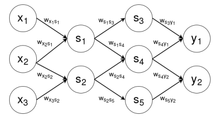
An example graph for an ANN computing a two dimensional output \(\vec{y}\) on a three dimensional input \(\vec{x}\) using five sigmoidal units \(s_1, \dots, s_5\) is shown below. An edge labeled with weight \(w_{ab}\) represents the component of the weight vector for node \(b\) that corresponds to the input coming from node \(a\). Note that this graph, because it has no cycles, is a feedforward neural network.

Layers

Thus, the above ANN would start by computing the outputs of nodes \(s_1\) and \(s_2\) given \(x_1\), \(x_2\), and \(x_3\). Once that was complete, the ANN would next compute the outputs of nodes \(s_3\), \(s_4\), and \(s_5\), dependent on the outputs of \(s_1\) and \(s_2\). Once that was complete, the ANN would do the final calculation of nodes \(y_1\) and \(y_2\), dependent on the outputs of nodes \(s_3\), \(s_4\), and \(s_5\).

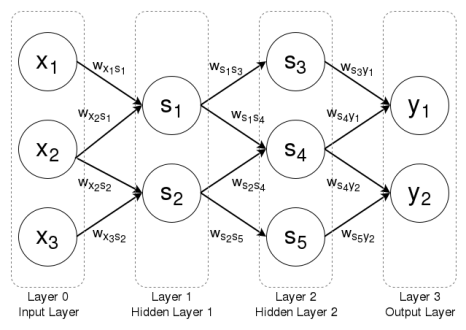
It is obvious from this computational flow that certain sets of nodes tend to be computed at the same time, since a different set of nodes uses their outputs as inputs. For example, set \(\{s_3, s_4, s_5\}\) depends on set \(\{s_1, s_2\}\). These sets of nodes that are computed together are known as layers, and ANNs are generally thought of a series of such layers, with each layer \(l_i\) dependent on previous layer \(l_{i-1}\) Thus, the above graph is composed of four layers. The first layer \(l_0\) is called the input layer (which does not need to be computed, since it is given), while the final layer \(l_3\) is called the output layer. The intermediate layers are known as hidden layers, which in this case are the layers \(l_1 = \{s_1, s_2\}\) and \(l_2 = \{s_3, s_4, s_5\}\), are usually numbered so that hidden layer \(h_i\) corresponds to layer \(l_i\). Thus, hidden layer \(h_1=\{s_1, s_2\}\) and hidden layer \(h_2=\{s_3, s_4, s_5\}\). The diagram below shows the example ANN with each node grouped into its appropriate layer.

The image source: Artificial Neural Network