Tuning the Hyperparameters and Layers of Neural Network Deep Learning

This article was published as a part of the Data Science Blogathon

Introduction

Bayesian Optimization: bayes_opt or hyperopt. That method can be applied to any kind of classification and regression Machine Learning algorithms for tabular data. However, Neural Network Deep Learning has a slightly different way to tune the hyperparameters (and the layers).

Neural Network is a Deep Learning technic to build a model according to training data to predict unseen data using many layers consisting of neurons. This is similar to other Machine Learning algorithms, except for the use of multiple layers. The use of multiple layers is what makes it Deep Learning.

Instead of directly building Machine Learning in 1 line, Neural Network requires users to build the architecture before compiling them into a model. Users will have to arrange how many layers and how many nodes or neurons to build. This is not found in other conventional Machine Learning algorithms.

I am sure that it is easy to find tutorials on the neural network on the internet. There are also many blogs explaining the concept behind a neural network. The code to perform hyperparameter-tuning to a neural network also can be found in many articles and shared notebooks. But, I feel it is quite rare to find a guide of neural network hyperparameter-tuning using Bayesian Optimization. The articles I found mostly depend on GridSearchCV or RandomizedSearchCV. Meanwhile, a neural network has many hyperparameters to tune. Bayesian optimization is more efficient in time and memory capacity for tuning many hyperparameters. I have described the reason in my past article.

Different datasets require different sets of hyperparameters to predict accurately. But, the large number of hyperparameters makes users difficult to decided which one to choose. There is no answer to how many layers are the most suitable, how many neurons are the best, or which optimizer suits the best for all datasets. Hyperparameter-tuning is important to find the possible best sets of hyperparameters to build the model from a specific dataset.

In this article, I will demonstrate the process to tune 2 things of Neural Network: (1) the hyperparameters and (2) the layers. I find it more difficult to find the latter tutorials than the former. The first one is the same as other conventional Machine Learning algorithms. The hyperparameters to tune are the number of neurons, activation function, optimizer, learning rate, batch size, and epochs. The second step is to tune the number of layers. This is what other conventional algorithms do not have. Different layers can affect the accuracy. Fewer layers may give an underfitting result while too many layers may make it overfitting.

For the hyperparameter-tuning demonstration, I use a dataset provided by Kaggle. I build a simple Multilayer Perceptron (MLP) neural network to do a binary classification task with prediction probability. The used package in Python is Keras built on top of Tensorflow. The dataset has an input dimension of 10. There are two hidden layers, followed by one output layer. The accuracy metric is the accuracy score. The callback of EarlyStopping is used to stop the learning process if there is no accuracy improvement in 20 epochs. Below is the illustration.

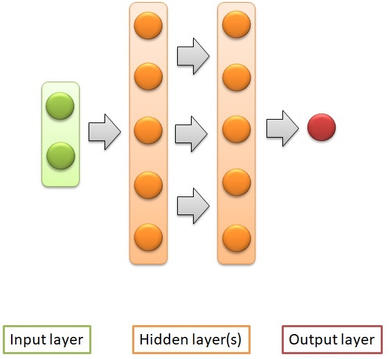
Fig. 1 MLP Neural Network to build. Source: created by myself

Hyperparameter Tuning in Deep Learning

The first hyperparameter to tune is the number of neurons in each hidden layer. In this case, the number of neurons in every layer is set to be the same. It also can be made different. The number of neurons should be adjusted to the solution complexity. The task with a more complex level to predict needs more neurons. The number of neurons range is set to be from 10 to 100.

An activation function is a parameter in each layer. Input data are fed to the input layer, followed by hidden layers, and the final output layer. The output layer contains the output value. The input values moving from a layer to another layer keep changing according to the activation function. The activation function decides how to compute the input values of a layer into output values. The output values of a layer are then passed to the next layer as input values again. The next layer then computes the values into output values for another layer again. There are 9 activation functions to tune in to this demonstration. Each activation function has its own formula (and graph) to compute the input values. It will not be discussed in this article.

The layers of a neural network are compiled and an optimizer is assigned. The optimizer is responsible to change the learning rate and weights of neurons in the neural network to reach the minimum loss function. Optimizer is very important to achieve the possible highest accuracy or minimum loss. There are 7 optimizers to choose from. Each has a different concept behind it.

One of the hyperparameters in the optimizer is the learning rate. We will also tune the learning rate. Learning rate controls the step size for a model to reach the minimum loss function. A higher learning rate makes the model learn faster, but it may miss the minimum loss function and only reach the surrounding of it. A lower learning rate gives a better chance to find a minimum loss function. As a tradeoff lower learning rate needs higher epochs, or more time and memory capacity resources.

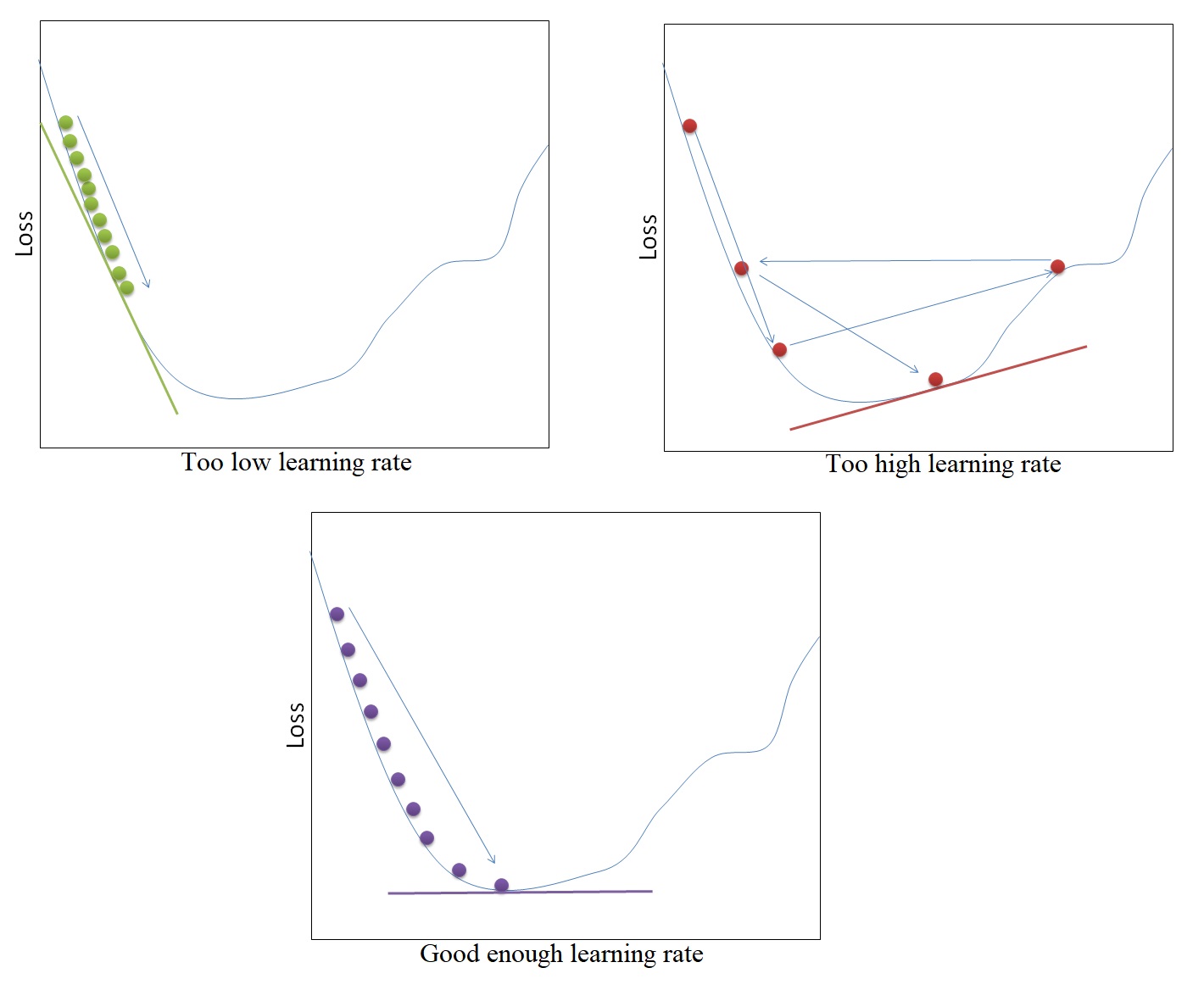
Fig 2. Learning rate illustration. Source: created by myself

If the observation size of the training dataset is too large, it will definitely take a longer time to build the model. To make the model learn faster, we can assign batch size so that not all of the training data are given to the model at the same time. Batch size is the number of training data sub-samples for the input. If the training dataset has 77,500 observations and the batch size is 1000, the model will learn 77 times with 1000 training data sub-samples and another last learning from the 500 training data sub-samples. The smaller batch size makes the learning process faster, but the variance of the validation dataset accuracy is higher. A bigger batch size has a slower learning process, but the validation dataset accuracy has a lower variance.

The number of times a whole dataset is passed through the neural network model is called an epoch. One epoch means that the training dataset is passed forward and backward through the neural network once. A too-small number of epochs results in underfitting because the neural network has not learned much enough. The training dataset needs to pass multiple times or multiple epochs are required. On the other hand, too many epochs will lead to overfitting where the model can predict the data very well, but cannot predict new unseen data well enough. The number of epoch must be tuned to gain the optimal result. This demonstration searches for a suitable number of epochs between 20 to 100.

Below is the code to tune the hyperparameters of a neural network as described above using Bayesian Optimization. The tuning searches for the optimum hyperparameters based on 5-fold cross-validation. The following code imports useful packages for Neural Network modeling.

# Import packages
import numpy as np
import pandas as pd
import matplotlib.pyplot as plt
import seaborn as sns
from sklearn.model_selection import train_test_split
from sklearn.model_selection import cross_val_score
from keras.models import Sequential
from keras.layers import Dense, BatchNormalization, Dropout
from keras.optimizers import Adam, SGD, RMSprop, Adadelta, Adagrad, Adamax, Nadam, Ftrl
from keras.callbacks import EarlyStopping, ModelCheckpoint
from keras.wrappers.scikit_learn import KerasClassifier
from math import floor
from sklearn.metrics import make_scorer, accuracy_score
from bayes_opt import BayesianOptimization
from sklearn.model_selection import StratifiedKFold
from keras.layers import LeakyReLU
LeakyReLU = LeakyReLU(alpha=0.1)
import warnings
warnings.filterwarnings('ignore')
pd.set_option("display.max_columns", None)

This code makes accuracy the scorer metric.

# Make scorer accuracy
score_acc = make_scorer(accuracy_score)

This code loads training and test datasets. It then splits the dataset into another training dataset and validation dataset. The validation dataset is 20% of the total dataset. The dataset is split according to the target variable.

# Load dataset
trainSet = pd.read_csv('../input/tabular-playground-series-apr-2021/train.csv')
# Feature generation: training data
train = trainSet.drop(columns=['Name', 'Ticket', 'Cabin'])
train = train.dropna(axis=0)
train = pd.get_dummies(train)
# train validation split
X_train, X_val, y_train, y_val = train_test_split(train.drop(columns=['PassengerId','Survived'], axis=0),
                                                  train['Survived'],
                                                  test_size=0.2, random_state=111,
                                                  stratify=train['Survived'])

The following code creates the objective function containing the Neural Network model. The function will return returns the score of the cross-validation.

# Create function
def nn_cl_bo(neurons, activation, optimizer, learning_rate,  batch_size, epochs ):
    optimizerL = ['SGD', 'Adam', 'RMSprop', 'Adadelta', 'Adagrad', 'Adamax', 'Nadam', 'Ftrl','SGD']
    optimizerD= {'Adam':Adam(lr=learning_rate), 'SGD':SGD(lr=learning_rate),
                 'RMSprop':RMSprop(lr=learning_rate), 'Adadelta':Adadelta(lr=learning_rate),
                 'Adagrad':Adagrad(lr=learning_rate), 'Adamax':Adamax(lr=learning_rate),
                 'Nadam':Nadam(lr=learning_rate), 'Ftrl':Ftrl(lr=learning_rate)}
    activationL = ['relu', 'sigmoid', 'softplus', 'softsign', 'tanh', 'selu',
                   'elu', 'exponential', LeakyReLU,'relu']
    neurons = round(neurons)
    activation = activationL[round(activation)]
    batch_size = round(batch_size)
    epochs = round(epochs)
    def nn_cl_fun():
        opt = Adam(lr = learning_rate)
        nn = Sequential()
        nn.add(Dense(neurons, input_dim=10, activation=activation))
        nn.add(Dense(neurons, activation=activation))
        nn.add(Dense(1, activation='sigmoid'))
        nn.compile(loss='binary_crossentropy', optimizer=opt, metrics=['accuracy'])
        return nn
    es = EarlyStopping(monitor='accuracy', mode='max', verbose=0, patience=20)
    nn = KerasClassifier(build_fn=nn_cl_fun, epochs=epochs, batch_size=batch_size,
                         verbose=0)
    kfold = StratifiedKFold(n_splits=5, shuffle=True, random_state=123)
    score = cross_val_score(nn, X_train, y_train, scoring=score_acc, cv=kfold, fit_params={'callbacks':[es]}).mean()
    return score

The code below sets the range of hyperparameters and run the Bayesian Optimization

# Set paramaters
params_nn ={
    'neurons': (10, 100),
    'activation':(0, 9),
    'optimizer':(0,7),
    'learning_rate':(0.01, 1),
    'batch_size':(200, 1000),
    'epochs':(20, 100)
}
# Run Bayesian Optimization
nn_bo = BayesianOptimization(nn_cl_bo, params_nn, random_state=111)
nn_bo.maximize(init_points=25, n_iter=4)

Output:

|   iter    |  target   | activa... | batch_... |  epochs   | learni... |  neurons  | optimizer |
-------------------------------------------------------------------------------------------------
|  1        |  0.5431   |  5.51     |  335.3    |  54.88    |  0.7716   |  36.58    |  1.044    |
|  2        |  0.5719   |  0.2023   |  536.2    |  39.09    |  0.3443   |  99.16    |  1.664    |
|  3        |  0.5432   |  0.7307   |  735.7    |  69.7     |  0.2815   |  51.96    |  0.8286   |
|  4        |  0.5431   |  0.6656   |  920.6    |  83.52    |  0.8422   |  83.37    |  6.937    |
|  5        |  0.7682   |  5.195    |  851.0    |  53.71    |  0.03717  |  50.87    |  0.7373   |
|  6        |  0.5719   |  7.355    |  758.2    |  65.22    |  0.2815   |  99.86    |  0.9663   |
|  7        |  0.6107   |  5.539    |  588.0    |  52.4     |  0.7306   |  39.05    |  2.804    |
|  8        |  0.5706   |  2.871    |  957.8    |  93.5     |  0.8157   |  13.07    |  6.604    |
|  9        |  0.5719   |  8.554    |  845.3    |  58.5     |  0.9671   |  47.53    |  2.232    |
|  10       |  0.6818   |  0.148    |  230.5    |  24.25    |  0.1367   |  13.0     |  1.585    |
|  11       |  0.6759   |  4.895    |  342.9    |  34.35    |  0.1581   |  71.47    |  3.283    |
|  12       |  0.5719   |  6.914    |  735.1    |  55.3     |  0.5993   |  51.55    |  6.743    |
|  13       |  0.5719   |  1.33     |  925.5    |  59.83    |  0.5966   |  71.62    |  1.242    |
|  14       |  0.6751   |  7.782    |  585.7    |  25.55    |  0.3711   |  42.54    |  3.304    |
|  15       |  0.5719   |  1.615    |  340.2    |  95.93    |  0.6591   |  22.15    |  6.495    |
|  16       |  0.6822   |  7.576    |  242.2    |  36.29    |  0.8738   |  70.65    |  2.081    |
|  17       |  0.5719   |  6.61     |  694.7    |  36.84    |  0.804    |  15.32    |  2.158    |
|  18       |  0.5719   |  1.866    |  977.8    |  92.75    |  0.6797   |  20.37    |  6.706    |
|  19       |  0.5144   |  0.8254   |  703.8    |  92.23    |  0.3464   |  68.75    |  6.476    |
|  20       |  0.5258   |  3.366    |  817.1    |  91.69    |  0.624    |  23.6     |  2.624    |
|  21       |  0.5815   |  5.723    |  567.3    |  62.58    |  0.3588   |  69.39    |  3.336    |
|  22       |  0.4856   |  4.091    |  299.8    |  53.0     |  0.2804   |  41.21    |  6.821    |
|  23       |  0.5719   |  1.94     |  746.3    |  22.54    |  0.837    |  73.15    |  6.762    |
|  24       |  0.7661   |  5.326    |  373.9    |  77.54    |  0.04056  |  47.68    |  1.969    |
|  25       |  0.6843   |  0.9562   |  541.1    |  87.25    |  0.1193   |  98.8     |  1.633    |
|  26       |  0.6839   |  7.588    |  234.1    |  72.25    |  0.4108   |  27.87    |  4.56     |
|  27       |  0.5719   |  3.724    |  412.4    |  62.06    |  0.9792   |  77.42    |  4.245    |
|  28       |  0.5719   |  1.738    |  997.2    |  48.97    |  0.7989   |  46.98    |  6.493    |
|  29       |  0.5719   |  8.671    |  828.0    |  51.03    |  0.8384   |  55.77    |  6.071    |

Here are the best hyperparameters.

params_nn_ = nn_bo.max['params']
activationL = ['relu', 'sigmoid', 'softplus', 'softsign', 'tanh', 'selu',
               'elu', 'exponential', LeakyReLU,'relu']
params_nn_['activation'] = activationL[round(params_nn_['activation'])]
params_nn_

Output:

{'activation': 'selu',
 'batch_size': 851.0135336291902,
 'epochs': 53.7054301919375,
 'learning_rate': 0.037173480215022196,
 'neurons': 50.872297884262295,
 'optimizer': 0.7372825972056519}

In the code above, the neural network is built in line 14 to line 24 of the #Create function starting from the function def nl_cl_fun. The neural network layers architecture is built before performing the cross-validation. This is different from conventional Machine Learning. Other Machine Learning does need to build the architecture like in def nl_cl_fun before performing the cross-validation.

Tune the Layers

Layers in Neural Network also determine the result of the prediction model. A smaller number of layers is enough for a simpler problem, but a larger number of layers is needed to build a model for a more complicated problem. The number of layers can be tuned using the “for loop” iteration. This demonstration tune the number of layers two times. Each time, the number of layers is tuned between 1 to 3.

Inserting regularization layers in a neural network can help prevent overfitting. This demonstration tries to tune whether to add regularization layers or not. There are two regularization layers to use here.

Batch normalization is placed after the first hidden layers. The batch normalization layer normalizes the values passed to it for every batch. This is similar to standard scaler in conventional Machine Learning.

Another regularization layer is the Dropout layer. The dropout layer, as its name suggests, randomly drops a certain number of neurons in a layer. The dropped neurons are not used anymore. The rate of how much percentage of neurons to drop is set in the dropout rate. The following is the code to tune the hyperparameters and layers at the same time.

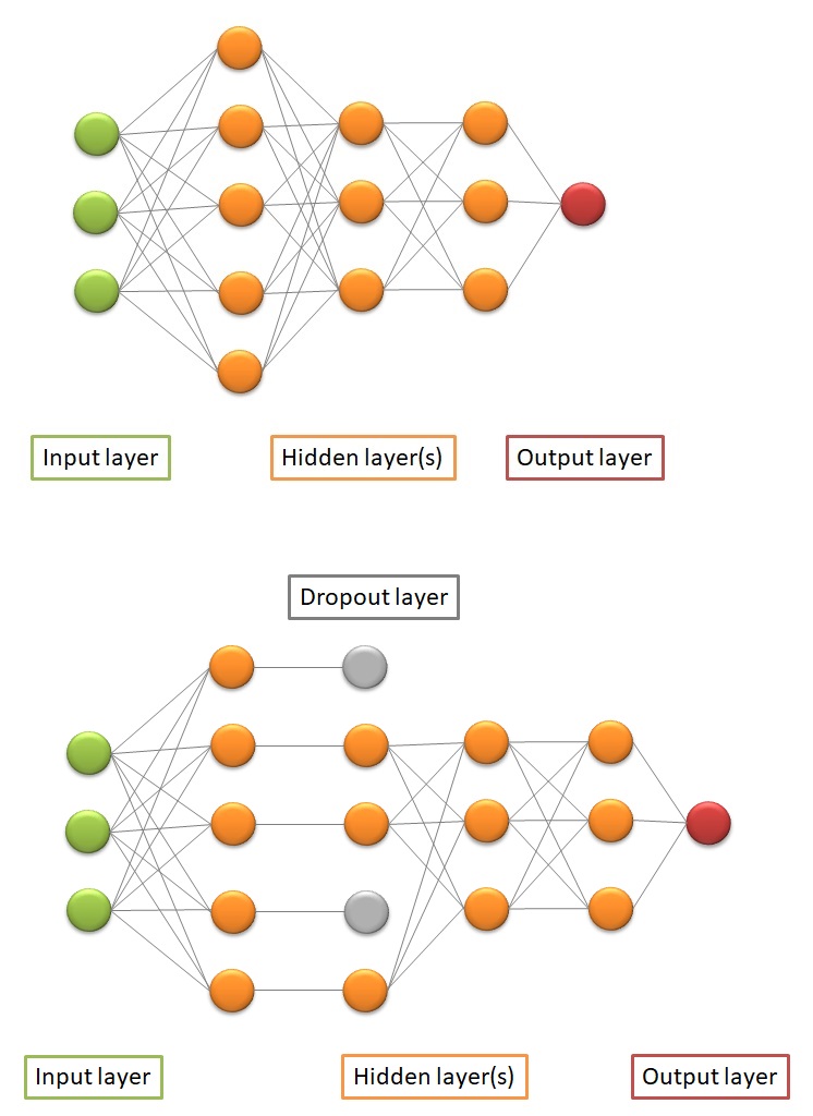Fig. 3 Dropout layer illustration. Source: created by myself

The following code creates a function for tuning the Neural Network hyperparameters and layers.

# Create function
def nn_cl_bo2(neurons, activation, optimizer, learning_rate, batch_size, epochs,
              layers1, layers2, normalization, dropout, dropout_rate):
    optimizerL = ['SGD', 'Adam', 'RMSprop', 'Adadelta', 'Adagrad', 'Adamax', 'Nadam', 'Ftrl','SGD']
    optimizerD= {'Adam':Adam(lr=learning_rate), 'SGD':SGD(lr=learning_rate),
                 'RMSprop':RMSprop(lr=learning_rate), 'Adadelta':Adadelta(lr=learning_rate),
                 'Adagrad':Adagrad(lr=learning_rate), 'Adamax':Adamax(lr=learning_rate),
                 'Nadam':Nadam(lr=learning_rate), 'Ftrl':Ftrl(lr=learning_rate)}
    activationL = ['relu', 'sigmoid', 'softplus', 'softsign', 'tanh', 'selu',
                   'elu', 'exponential', LeakyReLU,'relu']
    neurons = round(neurons)
    activation = activationL[round(activation)]
    optimizer = optimizerD[optimizerL[round(optimizer)]]
    batch_size = round(batch_size)
    epochs = round(epochs)
    layers1 = round(layers1)
    layers2 = round(layers2)
    def nn_cl_fun():
        nn = Sequential()
        nn.add(Dense(neurons, input_dim=10, activation=activation))
        if normalization > 0.5:
            nn.add(BatchNormalization())
        for i in range(layers1):
            nn.add(Dense(neurons, activation=activation))
        if dropout > 0.5:
            nn.add(Dropout(dropout_rate, seed=123))
        for i in range(layers2):
            nn.add(Dense(neurons, activation=activation))
        nn.add(Dense(1, activation='sigmoid'))
        nn.compile(loss='binary_crossentropy', optimizer=optimizer, metrics=['accuracy'])
        return nn
    es = EarlyStopping(monitor='accuracy', mode='max', verbose=0, patience=20)
    nn = KerasClassifier(build_fn=nn_cl_fun, epochs=epochs, batch_size=batch_size, verbose=0)
    kfold = StratifiedKFold(n_splits=5, shuffle=True, random_state=123)
    score = cross_val_score(nn, X_train, y_train, scoring=score_acc, cv=kfold, fit_params={'callbacks':[es]}).mean()
    return score

The following code searches for the optimum hyperparameters and layers for the Neural Network model.

params_nn2 ={
    'neurons': (10, 100),
    'activation':(0, 9),
    'optimizer':(0,7),
    'learning_rate':(0.01, 1),
    'batch_size':(200, 1000),
    'epochs':(20, 100),
    'layers1':(1,3),
    'layers2':(1,3),
    'normalization':(0,1),
    'dropout':(0,1),
    'dropout_rate':(0,0.3)
}
# Run Bayesian Optimization
nn_bo = BayesianOptimization(nn_cl_bo2, params_nn2, random_state=111)
nn_bo.maximize(init_points=25, n_iter=4)

Output:

|   iter    |  target   | activa... | batch_... |  dropout  | dropou... |  epochs   |  layers1  |  layers2  | learni... |  neurons  | normal... | optimizer |
-------------------------------------------------------------------------------------------------------------------------------------------------------------
|  1        |  0.6293   |  5.51     |  335.3    |  0.4361   |  0.2308   |  43.63    |  1.298    |  1.045    |  0.426    |  31.48    |  0.3377   |  6.935    |
|  2        |  0.6502   |  2.14     |  265.0    |  0.6696   |  0.1864   |  41.94    |  1.932    |  1.237    |  0.08322  |  91.07    |  0.794    |  5.884    |
|  3        |  0.5719   |  7.337    |  992.8    |  0.5773   |  0.2441   |  53.71    |  1.055    |  1.908    |  0.1143   |  83.55    |  0.6977   |  3.957    |
|  4        |  0.5886   |  2.468    |  998.8    |  0.138    |  0.1846   |  58.8     |  1.81     |  2.456    |  0.3296   |  46.05    |  0.319    |  6.631    |
|  5        |  0.5719   |  8.268    |  851.1    |  0.03408  |  0.283    |  96.04    |  2.613    |  1.963    |  0.9671   |  47.53    |  0.3188   |  0.1151   |
|  6        |  0.768    |  0.3436   |  242.5    |  0.128    |  0.01001  |  38.11    |  2.088    |  1.357    |  0.1876   |  23.47    |  0.683    |  3.283    |
|  7        |  0.5719   |  6.914    |  735.1    |  0.4413   |  0.1786   |  56.93    |  2.927    |  1.296    |  0.9077   |  54.81    |  0.5925   |  4.793    |
|  8        |  0.767    |  1.597    |  891.7    |  0.4821   |  0.0208   |  49.18    |  1.723    |  1.944    |  0.1877   |  25.78    |  0.9491   |  4.59     |
|  9        |  0.5432   |  1.215    |  942.2    |  0.8418   |  0.01583  |  36.29    |  2.745    |  2.348    |  0.3043   |  76.1     |  0.6183   |  1.473    |
|  10       |  0.5719   |  7.219    |  247.3    |  0.3082   |  0.06221  |  97.78    |  2.819    |  2.353    |  0.124    |  96.22    |  0.09171  |  4.409    |
|  11       |  0.5892   |  8.126    |  471.8    |  0.6528   |  0.2775   |  49.92    |  2.543    |  2.792    |  0.624    |  23.6     |  0.3749   |  4.451    |
|  12       |  0.5719   |  4.132    |  625.8    |  0.3523   |  0.198    |  58.12    |  1.909    |  1.25     |  0.4183   |  34.58    |  0.3467   |  6.821    |
|  13       |  0.7683   |  1.94     |  746.3    |  0.03181  |  0.2506   |  76.13    |  2.932    |  2.184    |  0.2252   |  74.73    |  0.03087  |  2.931    |
|  14       |  0.5764   |  2.531    |  285.0    |  0.4263   |  0.2522   |  28.83    |  2.973    |  1.467    |  0.7242   |  69.48    |  0.07776  |  4.881    |
|  15       |  0.768    |  2.388    |  921.5    |  0.8183   |  0.1198   |  85.62    |  1.396    |  2.045    |  0.4184   |  93.33    |  0.8254   |  3.507    |
|  16       |  0.7684   |  1.051    |  209.3    |  0.9132   |  0.1537   |  87.45    |  1.19     |  2.607    |  0.07161  |  67.19    |  0.9688   |  2.782    |
|  17       |  0.5144   |  5.936    |  371.9    |  0.8899   |  0.296    |  79.09    |  2.283    |  1.504    |  0.4811   |  34.13    |  0.8683   |  1.868    |
|  18       |  0.5719   |  8.757    |  370.8    |  0.2978   |  0.221    |  21.03    |  1.06     |  2.468    |  0.5033   |  29.63    |  0.00893  |  5.955    |
|  19       |  0.7635   |  4.828    |  778.8    |  0.6616   |  0.2516   |  51.06    |  1.852    |  2.656    |  0.4743   |  83.8     |  0.01418  |  2.777    |
|  20       |  0.5144   |  1.155    |  294.5    |  0.206    |  0.2243   |  94.41    |  1.761    |  1.921    |  0.8746   |  83.31    |  0.02497  |  6.111    |
|  21       |  0.5442   |  5.441    |  613.2    |  0.5893   |  0.2399   |  33.86    |  1.374    |  1.516    |  0.06056  |  59.74    |  0.3518   |  6.419    |
|  22       |  0.767    |  4.289    |  283.6    |  0.1525   |  0.08206  |  82.52    |  1.786    |  2.598    |  0.4387   |  17.34    |  0.01064  |  3.016    |
|  23       |  0.7437   |  5.966    |  612.2    |  0.5801   |  0.1479   |  79.24    |  2.579    |  2.562    |  0.1363   |  94.61    |  0.8777   |  4.897    |
|  24       |  0.6826   |  8.432    |  739.0    |  0.5944   |  0.1035   |  26.69    |  2.159    |  1.035    |  0.5569   |  66.93    |  0.6784   |  1.194    |
|  25       |  0.576    |  5.194    |  364.8    |  0.2515   |  0.2908   |  91.73    |  1.246    |  2.762    |  0.9485   |  51.39    |  0.413    |  4.04     |
|  26       |  0.6123   |  0.8666   |  764.0    |  0.09547  |  0.2738   |  71.59    |  2.418    |  2.742    |  0.01     |  89.31    |  0.0      |  1.49     |
|  27       |  0.7422   |  6.366    |  780.2    |  0.6271   |  0.1646   |  53.26    |  1.954    |  2.228    |  0.6962   |  81.66    |  0.1557   |  2.563    |
|  28       |  0.5144   |  4.821    |  779.7    |  0.8649   |  0.1344   |  37.63    |  2.574    |  1.528    |  0.3698   |  79.91    |  0.7947   |  5.56     |
|  29       |  0.5719   |  0.509    |  920.4    |  0.6302   |  0.2337   |  83.36    |  2.121    |  2.895    |  0.9025   |  99.29    |  0.8399   |  6.796    |

Here are the tuned hyperparameters and layers.

params_nn_ = nn_bo.max['params']
learning_rate = params_nn_['learning_rate']
activationL = ['relu', 'sigmoid', 'softplus', 'softsign', 'tanh', 'selu',
               'elu', 'exponential', LeakyReLU,'relu']
params_nn_['activation'] = activationL[round(params_nn_['activation'])]
params_nn_['batch_size'] = round(params_nn_['batch_size'])
params_nn_['epochs'] = round(params_nn_['epochs'])
params_nn_['layers1'] = round(params_nn_['layers1'])
params_nn_['layers2'] = round(params_nn_['layers2'])
params_nn_['neurons'] = round(params_nn_['neurons'])
optimizerL = ['Adam', 'SGD', 'RMSprop', 'Adadelta', 'Adagrad', 'Adamax', 'Nadam', 'Ftrl','Adam']
optimizerD= {'Adam':Adam(lr=learning_rate), 'SGD':SGD(lr=learning_rate),
             'RMSprop':RMSprop(lr=learning_rate), 'Adadelta':Adadelta(lr=learning_rate),
             'Adagrad':Adagrad(lr=learning_rate), 'Adamax':Adamax(lr=learning_rate),
             'Nadam':Nadam(lr=learning_rate), 'Ftrl':Ftrl(lr=learning_rate)}
params_nn_['optimizer'] = optimizerD[optimizerL[round(params_nn_['optimizer'])]]
params_nn_

Output:

{'activation': 'sigmoid',
 'batch_size': 209,
 'dropout': 0.9131504384208619,
 'dropout_rate': 0.15371924329624512,
 'epochs': 87,
 'layers1': 1,
 'layers2': 3,
 'learning_rate': 0.07160587078837888,
 'neurons': 67,
 'normalization': 0.9687811501818422,
 'optimizer': <tensorflow.python.keras.optimizer_v2.adadelta.Adadelta at 0x7fa6556fad10>}

It has 67 neurons for each layer. There is a batch normalization after the first hidden layer, followed by 1 neuron hidden layer. Next, the Dropout layer drops 15% of the neurons before the values are passed to 3 more neuron hidden layers. Finally, the output layer has one neuron containing the probability value. See Figure 4 for the illustration. Now that we have the optimal hyperparameters and layers with the estimated accuracy of 0.7684, let’s fit it into the training dataset. Eventually, we get an accuracy of 0.7681 for the validation dataset. The notebook for this article is made available here.

# Fitting Neural Network
def nn_cl_fun():
nn = Sequential()
nn.add(Dense(params_nn_['neurons'], input_dim=10, activation=params_nn_['activation']))
    if params_nn_['normalization'] > 0.5:
nn.add(BatchNormalization())
    for i in range(params_nn_['layers1']):
nn.add(Dense(params_nn_['neurons'], activation=params_nn_['activation']))
    if params_nn_['dropout'] > 0.5:
nn.add(Dropout(params_nn_['dropout_rate'], seed=123))
    for i in range(params_nn_['layers2']):
nn.add(Dense(params_nn_['neurons'], activation=params_nn_['activation']))
nn.add(Dense(1, activation='sigmoid'))
nn.compile(loss='binary_crossentropy', optimizer=params_nn_['optimizer'], metrics=['accuracy'])
    return nn
es = EarlyStopping(monitor='accuracy', mode='max', verbose=0, patience=20)
nn = KerasClassifier(build_fn=nn_cl_fun, epochs=params_nn_['epochs'], batch_size=params_nn_['batch_size'],
                         verbose=0)
 nn.fit(X_train, y_train, validation_data=(X_val, y_val), verbose=1)

Output:

Epoch 1/87
369/369 [==============================] - 2s 4ms/step - loss: 0.6859 - accuracy: 0.5540 - val_loss: 0.6825 - val_accuracy: 0.5719
Epoch 2/87
369/369 [==============================] - 1s 3ms/step - loss: 0.6822 - accuracy: 0.5723 - val_loss: 0.6818 - val_accuracy: 0.5719
Epoch 3/87
369/369 [==============================] - 1s 3ms/step - loss: 0.6819 - accuracy: 0.5711 - val_loss: 0.6810 - val_accuracy: 0.5719
. . .
Epoch 87/87
369/369 [==============================] - 1s 4ms/step - loss: 0.4993 - accuracy: 0.7683 - val_loss: 0.4940 - val_accuracy: 0.7681
<tensorflow.python.keras.callbacks.History at 0x7fa67610c750>

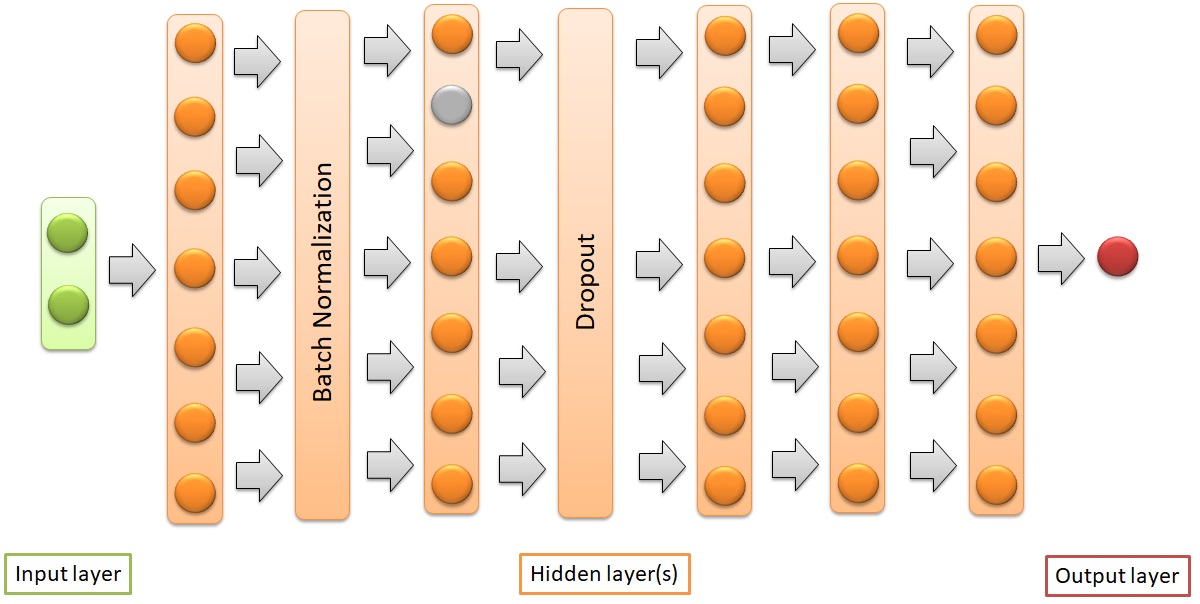Fig. 4 Illustration of the final model. Source: created by myself

About Author

Connect with me here.

The media shown in this article are not owned by Analytics Vidhya and is used at the Author’s discretion.

Related