Social Network Analysis & Mapping in Python with NetworkX

Mục Lục

Asymmetric Networks

What if the relationship between nodes is ‘child of’, then the relationship is no longer symmetric. If A is the child of B, then B is not a child of A. Such a network where the relationship is asymmetric (A is related to B, does not necessarily means that B is associated with A) is called an Asymmetric network. We can build the asymmetric network in NetworkX using DiGraph method, which is short of Directional Graph. Let us make an asymmetric graph.

G_asymmetric = nx.DiGraph()
G_asymmetric.add_edge('A','B')
G_asymmetric.add_edge('A','D')
G_asymmetric.add_edge('C','A')
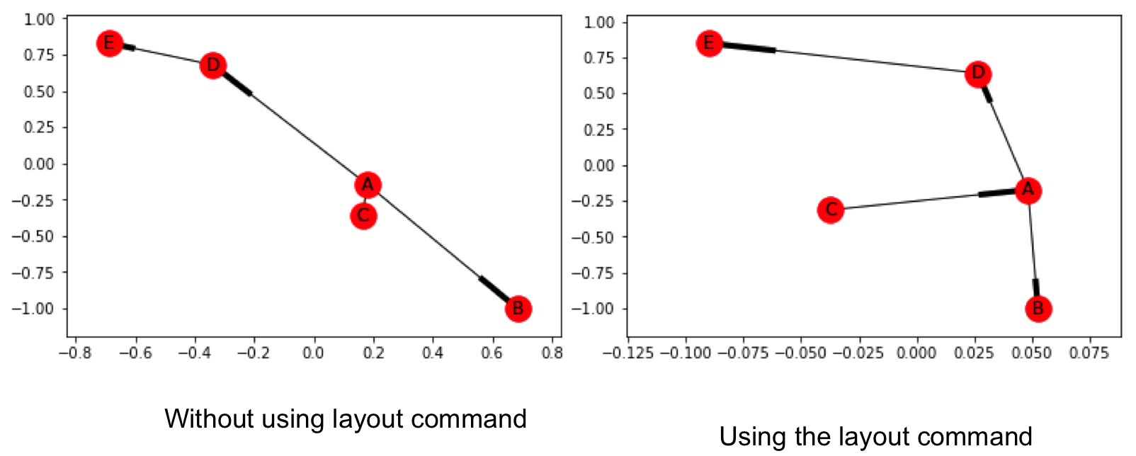
G_asymmetric.add_edge('D','E')

Now we visualize it. We can use the draw_networkx() function as before. However, it is possible that nodes do not separate out and are distinctly visible in the network drawn. To take care of this, we can use the function to force a layout, which positions the nodes in a manner that we can distinctly see them. We can accomplish this using spring_layout() function, followed by the draw_networkx() function.

nx.spring_layout(G_asymmetric)
nx.draw_networkx(G_asymmetric)

Below you can see the network with and without using the layout command. The one made using the layout command has more clarity.

visualized network 2

Weighted Networks

Till now we had networks without weights, but it is possible that networks are made with weights, for example, if in our initial network we consider the number of movies done together as a weight, we will get a Weighted Network. Let us make one again of the actors, but this time we add weight to the network, each edge has a weight signifying the number of movies they have done together.

G_weighted = nx.Graph()
G_weighted.add_edge('Amitabh Bachchan','Abhishek Bachchan', weight=25)
G_weighted.add_edge('Amitabh Bachchan','Aaamir Khan', weight=8)
G_weighted.add_edge('Amitabh Bachchan','Akshay Kumar', weight=11)
G_weighted.add_edge('Amitabh Bachchan','Dev Anand', weight=1)
G_weighted.add_edge('Abhishek Bachchan','Aaamir Khan', weight=4)
G_weighted.add_edge('Abhishek Bachchan','Akshay Kumar',weight=7)
G_weighted.add_edge('Abhishek Bachchan','Dev Anand', weight=1)
G_weighted.add_edge('Dev Anand','Aaamir Khan',weight=1)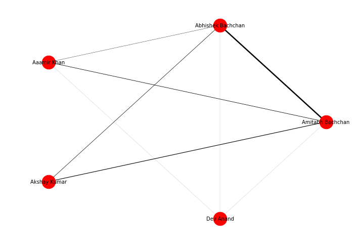

weighted network

The figure above shows the weighted network of actors in a circular layout. The edge width specifies the weight between two nodes.

Multigraph

We can give different attributes to the edges. For example, we can define a relation of neighbor between two nodes ‘A’ and ‘B’ using relation attribute. If within a network two nodes are connected with two different edges (relations) we have a multigraph. We can make a multigraph utilizing the MultiGraph class.

G = nx.MultiGraph()
G.add_edge('A','B',relation ='neighbor')
G.add_edge('A','B',relation='friend)
G.add_edge('B','C', relation='neighbor')
G.add_edge('D','C',relation='friend')

This code will construct a graph with two edges between A and B. We can check the connections using G.edges(), the output would show:

MultiEdgeDataView([('A', 'B', {'relation': 'neighbor'}), ('A', 'B', {'relation': 'friend'}), ('B', 'C', {'relation': 'neighbor'}), ('B', 'D', {'relation': 'neighbor'}), ('C', 'D', {'relation': 'friend'})])

Network Connectivity

Now the network is made, can we know more about a particular node in the network? Well yes, let us explore some of them.

Degree

Degree of a node defines the number of connections a node has. NetworkX has the function degree which we can use to determine the degree of a node in the network.

nx.degree(G_symmetric, 'Dev Anand`)

This will return a value of 3, as Dev Anand has worked with only three actors in the network.

Clustering Coefficient

It is observed that people who share connections in a social network tend to form associations. In other words, there is a tendency in a social network to form clusters. We can determine the clusters of a node, Local Clustering Coefficient, which is the fraction of pairs of the node’s friends (that is connections) that are connected with each other. To determine the local clustering coefficient, we make use of nx.clustering(Graph, Node) function.

In the symmetric Actor-network, you will find that Dev Anand has a local clustering coefficient of 1 and Abhishek Bachchan has a local clustering coefficient of 0.67.

The average clustering coefficient (sum of all the local clustering coefficients divided by the number of nodes) for the symmetric Actor-network is 0.867. We can obtain it using:

nx.average_clustering(G_symmetric)

Distance

We can also determine the shortest path between two nodes and its length in NetworkX using nx.shortest_path(Graph, Node1, Node2) and nx.shortest_path_length(Graph, Node1, Node2) functions respectively.

Executing

nx.shortest_path(G_symmetric, 'Dev Anand', 'Akshay Kumar')

Returns

['Dev Anand', 'Amitabh Bachchan', 'Akshay Kumar']

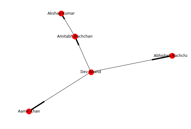
We can find the distance of a node from every other node in the network using breadth-first search algorithm, starting from that node. networkX provides the function bfs_tree to do it. And so if you try T = nx.bfs_tree(G_symmetric, 'Dev Anand') and now draw this tree, we will get a network structure telling how we can reach other nodes of the network starting from Dev Anand

nodes

Eccentricity

Eccentricity of a node A is defined as the largest distance between A and all other nodes. It can be found using nx.eccentricity() function. In the symmetric Actor-network, Dev Anand has an eccentricity of 2, and Abhishek Bachchan has an eccentricity of 1 (It is connected to all).

Network Influencers

Above we learned some of the network distance measures, they are useful in knowing how the information will spread through the network. In this section, we will learn how to find the most important nodes (individuals) in the network. These parameters are called as centrality measures.

Remember that popular girl from your high school or the schools top baseball player. These were the people who had the power to make your high school experience hell or heaven. What gave them this power? Centrality Measures can help us in identifying popularity, most liked, and biggest influencers within the network.

Degree Centrality

The people most popular or more liked usually are the ones who have more friends. Degree centrality is a measure of the number of connections a particular node has in the network. It is based on the fact that important nodes have many connections. NetworkX has the function degree_centrality() to calculate the degree centrality of all the nodes of a network.

Eigenvector Centrality

It is not just how many individuals one is connected too, but the type of people one is connected with that can decide the importance of a node. In Delhi Roads whenever the traffic police capture a person for breaking the traffic rule, the first sentence that traffic police hears is “Do you know whom I am related to?”.

Eigenvector centrality is a measure of exactly this. It decides that a node is important if it is connected to other important nodes. We can use the eigenvector_centrality() function of NetworkX to calculate eigenvector centrality of all the nodes in a network.

The Google’s Pagerank algorithm is a variant of Eigenvector centrality algorithm.

Betweenness Centrality

The Betweenness Centrality is the centrality of control. It represents the frequency at which a point occurs on the geodesic (shortest paths) that connected pair of points. It quantifies how many times a particular node comes in the shortest chosen path between two other nodes. The nodes with high betweenness centrality play a significant role in the communication/information flow within the network. The nodes with high betweenness centrality can have a strategic control and influence on others. An individual at such a strategic position can influence the whole group, by either withholding or coloring the information in transmission.

Networkx has the function betweenness_centrality() to measure it for the network. It has options to select if we want betweenness values to be normalized or not, weights to be included in centrality calculation or not, and to include the endpoints in the shortest path counts or not.

Combining it all

Let us start with the Facebook data, for our analysis here we will use Facebook combined ego networks dataset, it contains the aggregated network of ten individuals’ Facebook friends list. You can download the required facebook_combined.txt file from the Stanford University site.

You can get your own Facebook/Twitter data using the Facebook/Twitter APIs. Look forward to the next forthcoming tutorial where we will learn how to use Facebook and Twitter APIs to get data and use the information acquired here to analyze it.

We read in the file and construct the Graph:

G_fb = nx.read_edgelist("facebook_combined.txt", create_using = nx.Graph(), nodetype=int)

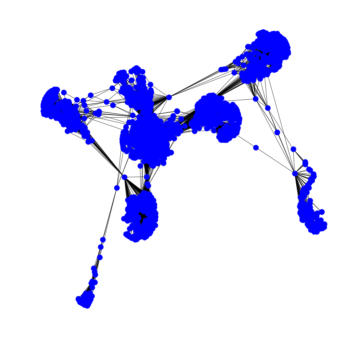
The network consists of 4,039 nodes, connected via 88,234 edges! Yep, it is a big network. You get the information using the info() function.

[In]: print(nx.info(G_fb))


[Out]: Name:
       Type: Graph
       Number of nodes: 4039
       Number of edges: 88234
       Average degree:  43.6910

Below you can see the network:

network

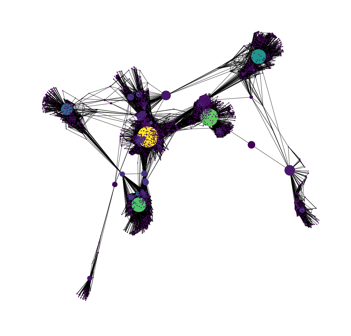
We can also visualize the network such that the node color varies with Degree and node size with Betweenness Centrality. The code to do this is:

pos = nx.spring_layout(G_fb)
betCent = nx.betweenness_centrality(G_fb, normalized=True, endpoints=True)
node_color = [20000.0 * G_fb.degree(v) for v in G_fb]
node_size =  [v * 10000 for v in betCent.values()]
plt.figure(figsize=(20,20))
nx.draw_networkx(G_fb, pos=pos, with_labels=False,
                 node_color=node_color,
                 node_size=node_size )
plt.axis('off')

And the resulting graph is:

resulting graph

You can also know the labels of the nodes with the highest betweenness centrality using:

sorted(betCent, key=betCent.get, reverse=True)[:5]

The table below lists the five node labels with the highest centrality measures.

Degree Centrality
Eigenvector Centrality
Betweenness Centrality

107
1912
107

1684
2266
1684

1912
2206
3437

3437
2233
1912

0
2464
1085

We can see that some nodes are common between Degree Centrality, which is a measure of degree, and Betweenness Centrality which controls the information flow. It is natural that nodes that are more connected also lie on shortest paths between other nodes. The node 1912 is an important node as it is crucial according to all three centrality measures that we had considered.