
Siamese networks with Keras, TensorFlow, and Deep Learning – PyImageSearch
In this tutorial you will learn how to implement and train siamese networks using Keras, TensorFlow, and Deep Learning.

This tutorial is part two in our three-part series on the fundamentals of siamese networks:
- Part #1: Building image pairs for siamese networks with Python (last week’s post)
- Part #2: Training siamese networks with Keras, TensorFlow, and Deep Learning (this week’s tutorial)
- Part #3: Comparing images using siamese networks (next week’s tutorial)
Using our siamese network implementation, we will be able to:
- Present two input images to our network.
- The network will predict whether or not these two images belong to the same class (i.e., verification).
- We’ll then be able to check the confidence score of the network to confirm the verification.
Practical, real-world use cases of siamese networks include face recognition, signature verification, prescription pill identification, and more!
Furthermore, siamese networks can be trained with astoundingly little data, making more advanced applications such as one-shot learning and few-shot learning possible.
To learn how to implement and train siamese networks with Keras and TenorFlow, just keep reading.
![]()
Mục Lục
Looking for the source code to this post?
Jump Right To The Downloads Section
Siamese networks with Keras, TensorFlow, and Deep Learning
In the first part of this tutorial, we will discuss siamese networks, how they work, and why you may want to use them in your own deep learning applications.
From there, you’ll learn how to configure your development environment such that you can follow along with this tutorial and learn how to train your own siamese networks.
We’ll then review our project directory structure and implement a configuration file, followed by three helper functions:
- A method used to generate image pairs such that we can train our siamese network
- A custom CNN layer to compute Euclidean distances between vectors inside of the network
- A utility used to plot the siamese network training history to disk
Given our helper utilities, we’ll implement our training script used to load the MNIST dataset from disk and train a siamese network on the data.
We’ll wrap up this tutorial with a discussion of our results.
What are siamese networks and how do they work?
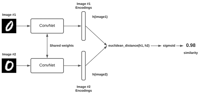 Figure 1: A basic siamese network architecture implementation accepts two input images (left), has identical CNN subnetworks for each input with each subnetwork ending in a fully-connected layer (middle), computes the Euclidean distance between the fully-connected layer outputs, and then passes the distance through a sigmoid activation function to determine similarity (right) (figure inspiration).
Last week’s tutorial covered the fundamentals of siamese networks, how they work, and what real-world applications are applicable to them. I’ll provide a quick review of them here, but I highly suggest that you read last week’s guide for a more in-depth review of siamese networks.
Figure 1 at the top of this section shows the basic architecture of a siamese network. You’ll immediately notice that the siamese network architecture is different from most standard classification architectures.
Notice how there are two inputs to the network along with two branches (i.e., “sister networks”). Each of these sister networks is identical to the other. The outputs of the two subnetworks are combined, and then the final output similarity score is returned.
To make this concept a bit more concrete, let’s break it down further in context of Figure 1 above:
- On the left we present two example digits (from the MNIST dataset) to the siamese model. Our goal is to determine if these digits belong to the same class or not.
- The middle shows the siamese network itself. These two subnetworks have the same architecture and same parameters, and they mirror each other — if the weights in one subnetwork are updated, then the weights in the other subnetwork(s) are updated as well.
- The output of each subnetwork is a fully-connected (FC) layer. We typically compute the Euclidean distance between these outputs and feed them through a sigmoid activation such that we can determine how similar the two input images are. The sigmoid activation function values closer to “1” imply more similar while values closer to “0” indicate “less similar.”
To actually train the siamese network architecture, we have a number of loss functions that we can utilize, including binary cross-entropy, triplet loss, and contrastive loss.
The latter two loss functions require image triplets (three input images to the network), which is different from the image pairs (two input images) that we are using today.
We’ll be using binary cross-entropy to train our siamese networks today. In the future I will cover intermediate/advanced siamese networks, including image triplets, triplet loss, and contrastive loss — but for now, let’s walk before we run.
Configuring your development environment
We’ll be using Keras and TensorFlow throughout this series of tutorials on siamese networks. I suggest you take the time to configure your deep learning development environment now.
I recommend you follow either of these two guides to install TensorFlow and Keras on your system (I recommend you install TensorFlow 2.3 for this guide):
Either tutorial will help you configure your system with all the necessary software for this blog post in a convenient Python virtual environment.
Having problems configuring your development environment?
 Figure 2: Having trouble configuring your dev environment? Want access to pre-configured Jupyter Notebooks running on Google Colab? Be sure to join PyImageSearch Plus —- you’ll be up and running with this tutorial in a matter of minutes.
All that said, are you:
- Short on time?
- Learning on your employer’s administratively locked system?
- Wanting to skip the hassle of fighting with the command line, package managers, and virtual environments?
- Ready to run the code right now on your Windows, macOS, or Linux system?
Then join PyImageSearch Plus today!
Gain access to Jupyter Notebooks for this tutorial and other PyImageSearch guides that are pre-configured to run on Google Colab’s ecosystem right in your web browser! No installation required.
And best of all, these Jupyter Notebooks will run on Windows, macOS, and Linux!
Project structure
Before we can train our siamese network, we first need to review our project directory structure.
Start by using the “Downloads” section of this tutorial to download the source code, pre-trained siamese network model, etc.
From there, let’s take a peek at what’s inside:
$ tree . --dirsfirst
.
├── output
│   ├── siamese_model
│   │   ├── variables
│   │   │   ├── variables.data-00000-of-00001
│   │   │   └── variables.index
│   │   └── saved_model.pb
│   └── plot.png
├── pyimagesearch
│   ├── config.py
│   ├── siamese_network.py
│   └── utils.py
└── train_siamese_network.py

2 directories, 6 files
Inside the pyimagesearch module we have three Python scripts:
config.pysiamese_network.pyutils.py
The train_siamese_network.py uses the three Python scripts in our pyimagesearch module to:
- Load the MNIST dataset from disk
- Create positive and negative image pairs from MNIST
- Build the siamese network architecture
- Train the siamese network on the image pairs
- Serialize the siamese network model and training history plot to our
outputdirectory
With our project directory structure reviewed, let’s move on to creating our configuration file.
Note: The pre-trained siamese_model included in the “Downloads” associated with this tutorial was created using TensorFlow 2.3. I recommend you use TensorFlow 2.3 for this guide. If you instead wish to use another version of TensorFlow, that’s perfectly okay, but you will need to execute train_siamese_network.py to train and serialize the model. You’ll also need to keep this model for next week’s tutorial when we use the trained siamese network to compare images.
Creating our siamese network configuration file
Our configuration file is short and sweet. Open up config.py, and insert the following code:
# import the necessary packages
import os

# specify the shape of the inputs for our network
IMG_SHAPE = (28, 28, 1)

# specify the batch size and number of epochs
BATCH_SIZE = 64
EPOCHS = 100
Line 5 initializes our input IMG_SHAPE spatial dimensions. Since we are working with the MNIST digits dataset, our images are 28×28 pixels with a single grayscale channel.
We then define our BATCH_SIZE and the total number of epochs we are training for.
In our own experiments we found that training for only 10 epochs yielded good results, but training for longer yielded higher accuracy. If you’re short on time, or if your machine doesn’t have a GPU, updating EPOCHS to 10 will still yield good results.
Next, let’s define our output paths:
# define the path to the base output directory
BASE_OUTPUT = "output"

# use the base output path to derive the path to the serialized
# model along with training history plot
MODEL_PATH = os.path.sep.join([BASE_OUTPUT, "siamese_model"])
PLOT_PATH = os.path.sep.join([BASE_OUTPUT, "plot.png"])
Line 12 initializes the BASE_OUTPUT path to be our output directory.
We then use the BASE_OUTPUT path to derive the path to our MODEL_PATH, which is our serialized Keras/TensorFlow model.
Since our siamese network implementation requires that we use a Lambda layer, we’ll be using SavedModel format, which according to the TensorFlow documentation, handles custom objects and implementations better.
The SavedModel format results in an output model directory containing the optimizer, losses, and metrics (saved_model.pb) along with the model weights themselves (stored in a variables/ directory).
Implementing the siamese network architecture with Keras and TensorFlow
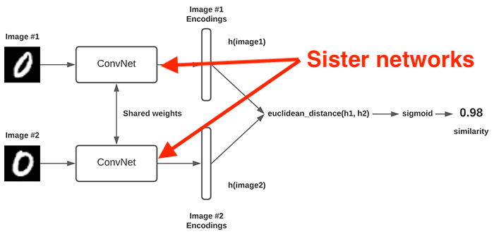 Figure 3: We’ll be implementing the basic ConvNet architecture used for our sister networks when building a siamese model.
A siamese network architecture consists of two or more sister networks (highlighted in Figure 3 above). Essentially, a sister network is a basic Convolutional Neural Network that results in a fully-connected (FC) layer, sometimes called an embedded layer.
When we go to construct the siamese network architecture itself, we will:
- Instantiate our sister networks
- Create a
Lambdalayer that computes the Euclidean distances between the outputs of the sister networks - Create an FC layer with a single node and a sigmoid activation function
The result will be a fully-constructed siamese network.
But before we get there, we first need to implement our sister network component of the siamese network architecture.
Open up siamese_network.py in your project directory structure, and let’s get to work:
# import the necessary packages
from tensorflow.keras.models import Model
from tensorflow.keras.layers import Input
from tensorflow.keras.layers import Conv2D
from tensorflow.keras.layers import Dense
from tensorflow.keras.layers import Dropout
from tensorflow.keras.layers import GlobalAveragePooling2D
from tensorflow.keras.layers import MaxPooling2D
We start on Lines 2-8 by importing our required Python packages. These imports should all feel pretty standard to you if you’ve ever trained a CNN with Keras/TensorFlow before.
If you need a refresher on CNNs, I recommend you read my Keras tutorial along with my book Deep Learning for Computer Vision with Python.
With our imports taken care of, we can now define the build_siamese_model function responsible for constructing the sister networks:
def build_siamese_model(inputShape, embeddingDim=48):
	# specify the inputs for the feature extractor network
	inputs = Input(inputShape)

	# define the first set of CONV => RELU => POOL => DROPOUT layers
	x = Conv2D(64, (2, 2), padding="same", activation="relu")(inputs)
	x = MaxPooling2D(pool_size=(2, 2))(x)
	x = Dropout(0.3)(x)

	# second set of CONV => RELU => POOL => DROPOUT layers
	x = Conv2D(64, (2, 2), padding="same", activation="relu")(x)
	x = MaxPooling2D(pool_size=2)(x)
	x = Dropout(0.3)(x)
Our build_siamese_model function accepts two parameters:
inputShapeembeddingDim
Line 12 initializes the input spatial dimensions to our sister network.
From there, Lines 15-22 define two sets of CONV => RELU => POOL layer sets. Each CONV layer learns a total of 64 2×2 filters. We then apply a ReLU activation function and apply max pooling with a 2×2 stride.
We can now finish constructing the sister network architecture:
	# prepare the final outputs
	pooledOutput = GlobalAveragePooling2D()(x)
	outputs = Dense(embeddingDim)(pooledOutput)

	# build the model
	model = Model(inputs, outputs)

	# return the model to the calling function
	return model
Line 25 applies global average pooling to the 7x7x64 volume (assuming a 28×28 input to the network), resulting in an output of 64-d.
We take this pooledOutput and then apply a fully-connected layer with the specified embeddingDim (Line 26) — this Dense layer serves as the output of the sister network.
Line 29 then builds the sister network Model, which is then returned to the calling function.
I’ve included a summary of the model below:
Model: "model"
_________________________________________________________________
Layer (type)                 Output Shape              Param #
=================================================================
input_3 (InputLayer)         [(None, 28, 28, 1)]       0
_________________________________________________________________
conv2d (Conv2D)              (None, 28, 28, 64)        320
_________________________________________________________________
max_pooling2d (MaxPooling2D) (None, 14, 14, 64)        0
_________________________________________________________________
dropout (Dropout)            (None, 14, 14, 64)        0
_________________________________________________________________
conv2d_1 (Conv2D)            (None, 14, 14, 64)        16448
_________________________________________________________________
max_pooling2d_1 (MaxPooling2 (None, 7, 7, 64)          0
_________________________________________________________________
dropout_1 (Dropout)          (None, 7, 7, 64)          0
_________________________________________________________________
global_average_pooling2d (Gl (None, 64)                0
_________________________________________________________________
dense (Dense)                (None, 48)                3120
=================================================================
Total params: 19,888
Trainable params: 19,888
Non-trainable params: 0
_________________________________________________________________
Here’s a quick review of the model we just constructed:
- Each sister network will accept a 28x28x1 input.
- We then apply a CONV layer to learn a total of 64 filters. Max pooling is applied with a 2×2 stride to reduce the spatial dimensions to 14x14x64.
- Another CONV layer (again, learning 64 filters) and POOL layer are applied, reducing the spatial dimensions further to 7x7x64.
- Global average pooling is applied to average the 7x7x64 volume down to 64-d.
- This 64-d pooling output is passed into an FC layer that has 48 nodes.
- The 48-d vector serves as the output of our sister network.
In the train_siamese_network.py script, you will learn how to instantiate two instances of our sister network and then finish constructing the siamese network architecture itself.
Implementing our pair generation, euclidean distance, and plot history utility functions
With our configuration file and sister network component of the siamese network architecture implemented, let’s now move on to our helper functions and methods located in the utils.py file of the pyimagesearch module.
Open up utils.py, and let’s review it:
# import the necessary packages
import tensorflow.keras.backend as K
import matplotlib.pyplot as plt
import numpy as np
We start off on Lines 2-4 importing our required Python packages.
We import our Keras/TensorFlow backend so that we can construct our custom Euclidean distance Lambda layer.
The matplotlib library will be used to create a helper function to plot our training history.
Next, we have our make_pairs function, which we discussed in detail last week:
def make_pairs(images, labels):
	# initialize two empty lists to hold the (image, image) pairs and
	# labels to indicate if a pair is positive or negative
	pairImages = []
	pairLabels = []

	# calculate the total number of classes present in the dataset
	# and then build a list of indexes for each class label that
	# provides the indexes for all examples with a given label
	numClasses = len(np.unique(labels))
	idx = [np.where(labels == i)[0] for i in range(0, numClasses)]

	# loop over all images
	for idxA in range(len(images)):
		# grab the current image and label belonging to the current
		# iteration
		currentImage = images[idxA]
		label = labels[idxA]

		# randomly pick an image that belongs to the *same* class
		# label
		idxB = np.random.choice(idx[label])
		posImage = images[idxB]

		# prepare a positive pair and update the images and labels
		# lists, respectively
		pairImages.append([currentImage, posImage])
		pairLabels.append([1])

		# grab the indices for each of the class labels *not* equal to
		# the current label and randomly pick an image corresponding
		# to a label *not* equal to the current label
		negIdx = np.where(labels != label)[0]
		negImage = images[np.random.choice(negIdx)]

		# prepare a negative pair of images and update our lists
		pairImages.append([currentImage, negImage])
		pairLabels.append([0])

	# return a 2-tuple of our image pairs and labels
	return (np.array(pairImages), np.array(pairLabels))
I’m not going to perform a full review of this function, as again, we covered in great detail in Part 1 of this series on siamese networks; however, the high-level gist is that:
- In order to train siamese networks, we need both positive and negative pairs
- A positive pair is two images that belong to the same class (i.e., two examples of the digit “8”)
- A negative pair is two images that belong to different classes (i.e., one image containing a “1” and the other image containing a “3”)
- The
make_pairsfunction accepts an input set ofimagesand associatedlabelsand then constructs these positive and negative image pairs for training, returning them to the calling function
For a more detailed review on the make_pairs function, refer to my tutorial Building image pairs for siamese networks with Python.
Our next function, euclidean_distance, accepts a 2-tuple of vectors and then computes the Euclidean distance between them, utilizing Keras/TensorFlow functions to do so:
def euclidean_distance(vectors):
	# unpack the vectors into separate lists
	(featsA, featsB) = vectors

	# compute the sum of squared distances between the vectors
	sumSquared = K.sum(K.square(featsA - featsB), axis=1,
		keepdims=True)

	# return the euclidean distance between the vectors
	return K.sqrt(K.maximum(sumSquared, K.epsilon()))
The euclidean_distance function accepts a single parameter, vectors, which are the outputs from the fully-connected layers of both our sister networks in the siamese network architecture.
We unpack the vectors into featsA and featsB (Line 50) and then compute the sum of squared differences between the vectors (Line 53 and 54).
We round out the function by taking the square root of the sum of squared differences, yielding the Euclidean distance (Line 57).
Take note that we are using Keras/TensorFlow functions to compute the Euclidean distance rather than using NumPy or SciPy.
Why is that?
Wouldn’t it just be simpler to use the Euclidean distance functions built into NumPy and SciPy?
Why go through all the hassle of reimplementing the Euclidean distance with Keras/TensorFlow?
The reason will become more clear once we get to the train_siamese_network.py script, but the gist is that in order to construct our siamese network architecture, we need to be able to compute the Euclidean distance between the sister network outputs inside the siamese architecture itself.
To accomplish this task we’ll use a custom Lambda layer that can be used to embed arbitrary Keras/TensorFlow functions inside of a model (hence why Keras/TensorFlow functions are used to implement the Euclidean distance).
Our final function, plot_training, accepts (1) the training history from calling model.fit and (2) an output plotPath:
def plot_training(H, plotPath):
	# construct a plot that plots and saves the training history
	plt.style.use("ggplot")
	plt.figure()
	plt.plot(H.history["loss"], label="train_loss")
	plt.plot(H.history["val_loss"], label="val_loss")
	plt.plot(H.history["accuracy"], label="train_acc")
	plt.plot(H.history["val_accuracy"], label="val_acc")
	plt.title("Training Loss and Accuracy")
	plt.xlabel("Epoch #")
	plt.ylabel("Loss/Accuracy")
	plt.legend(loc="lower left")
	plt.savefig(plotPath)
Given our training history variable, H, we plot both our training and validation loss and accuracy. The output plot is then saved to disk to plotPath.
Creating our siamese network training script with Keras and TensorFlow
We are now ready to implement our siamese network training script!
Inside train_siamese_network.py we will:
- Load the MNIST dataset from disk
- Construct our training and testing image pairs
- Create two instances of our
build_siamese_modelto serve as our sister networks - Finish constructing the siamese network architecture by piping the outputs of the sister networks through our custom
euclidean_distancefunction (using aLambdalayer) - Apply a sigmoid activation to the output of the Euclidean distance
- Train the siamese network architecture on our image pairs
It sounds like a complicated process, but we’ll be able to accomplish all of these tasks in under 60 lines of code!
Open up train_siamese_network.py, and let’s get to work:
# import the necessary packages
from pyimagesearch.siamese_network import build_siamese_model
from pyimagesearch import config
from pyimagesearch import utils
from tensorflow.keras.models import Model
from tensorflow.keras.layers import Dense
from tensorflow.keras.layers import Input
from tensorflow.keras.layers import Lambda
from tensorflow.keras.datasets import mnist
import numpy as np
Lines 2-10 import our required Python packages. Notable imports include:
build_siamese_modelconfigutilsLambda
With our imports taken care of, we can move on to loading the MNIST dataset from disk, preprocessing it, and constructing our image pairs:
# load MNIST dataset and scale the pixel values to the range of [0, 1]
print("[INFO] loading MNIST dataset...")
(trainX, trainY), (testX, testY) = mnist.load_data()
trainX = trainX / 255.0
testX = testX / 255.0

# add a channel dimension to the images
trainX = np.expand_dims(trainX, axis=-1)
testX = np.expand_dims(testX, axis=-1)

# prepare the positive and negative pairs
print("[INFO] preparing positive and negative pairs...")
(pairTrain, labelTrain) = utils.make_pairs(trainX, trainY)
(pairTest, labelTest) = utils.make_pairs(testX, testY)
Line 14 loads the MNIST digits dataset from disk.
We then preprocess the MNIST images by scaling them from the range [0, 255] to [0, 1] (Lines 15 and 16) and then adding a channel dimension (Lines 19 and 20).
We use our make_pairs function to create positive and negative image pairs for our training and testing sets, respectively (Lines 24 and 25). If you need a refresher on the make_pairs function, I suggest you read Part 1 of this series, which covers image pairs in detail.
Let’s now construct our siamese network architecture:
# configure the siamese network
print("[INFO] building siamese network...")
imgA = Input(shape=config.IMG_SHAPE)
imgB = Input(shape=config.IMG_SHAPE)
featureExtractor = build_siamese_model(config.IMG_SHAPE)
featsA = featureExtractor(imgA)
featsB = featureExtractor(imgB)
Lines 29-33 create our sister networks:
- First, we create two inputs, one for each image in the pair (Lines 29 and 30).
- Line 31 then builds the sister network architecture, which serves as
featureExtractor. - Each image in the pair will be passed through the
featureExtractor, resulting in a 48-d feature vector (Lines 32 and 33). Since there are two images in a pair, we thus have two 48-d feature vectors.
Perhaps you’re wondering why we didn’t call build_siamese_model twice? We have two sister networks in our architecture, right?
Well, keep in mind what you learned last week:
“These two sister networks have the same architecture and same parameters and mirror each other — if the weights in one subnetwork are updated, then the weights in the other network(s) are updated as well.”
So, even though there are two sister networks, we actually implement them as a single instance. Essentially, this single network is treated as a feature extractor (hence why we named it featureExtractor). The weights of the network are then updated via backpropagation as we train the network.
Let’s now finish constructing our siamese network architecture:
# finally, construct the siamese network
distance = Lambda(utils.euclidean_distance)([featsA, featsB])
outputs = Dense(1, activation="sigmoid")(distance)
model = Model(inputs=[imgA, imgB], outputs=outputs)
Line 36 utilizes a Lambda layer to compute the euclidean_distance between the featsA and featsB network (remember, these values are the outputs of passing each image in the pair through the sister network feature extractor).
We then apply a Dense layer with a single node with a sigmoid activation function applied to it.
The sigmoid activation function is used here because the output range of the function is [0, 1]. An output closer to 0 implies that the image pairs are less similar (and therefore from different classes), while a value closer to 1 implies they are more similar (and more likely to be from the same class).
Line 38 then constructs the siamese network Model. The inputs consist of our image pair, imgA and imgB. The outputs of the network is the sigmoid activation.
Now that our siamese network architecture is constructed, we can move on to training it:
# compile the model
print("[INFO] compiling model...")
model.compile(loss="binary_crossentropy", optimizer="adam",
	metrics=["accuracy"])

# train the model
print("[INFO] training model...")
history = model.fit(
	[pairTrain[:, 0], pairTrain[:, 1]], labelTrain[:],
	validation_data=([pairTest[:, 0], pairTest[:, 1]], labelTest[:]),
	batch_size=config.BATCH_SIZE,
	epochs=config.EPOCHS)
Lines 42 and 43 compile our siamese network using binary cross-entropy as our loss function.
We use binary cross-entropy here because this is essentially a two-class classification problem — given a pair of input images, we seek to determine how similar these two images are and, more specifically, if they are from the same or different class.
More advanced loss functions can be used here as well, including triplet loss and contrastive loss. I’ll be covering how to use these loss functions, including constructing image triplets, in a future series on the PyImageSearch blog (which will cover more advanced siamese networks).
Lines 47-51 then train the siamese network on the image pairs.
Once the model is trained, we can serialize it to disk and plot the training history:
# serialize the model to disk
print("[INFO] saving siamese model...")
model.save(config.MODEL_PATH)

# plot the training history
print("[INFO] plotting training history...")
utils.plot_training(history, config.PLOT_PATH)
Congrats on implementing our siamese network training script!
Training our siamese network with Keras and TensorFlow
We are now ready to train our siamese network using Keras and TensorFlow! Make sure you use the “Downloads” section of this tutorial to download the source code.
From there, open up a terminal, and execute the following command:
$ python train_siamese_network.py
[INFO] loading MNIST dataset...
[INFO] preparing positive and negative pairs...
[INFO] building siamese network...
[INFO] training model...
Epoch 1/100
1875/1875 [==============================] - 11s 6ms/step - loss: 0.6210 - accuracy: 0.6469 - val_loss: 0.5511 - val_accuracy: 0.7541
Epoch 2/100
1875/1875 [==============================] - 11s 6ms/step - loss: 0.5433 - accuracy: 0.7335 - val_loss: 0.4749 - val_accuracy: 0.7911
Epoch 3/100
1875/1875 [==============================] - 11s 6ms/step - loss: 0.5014 - accuracy: 0.7589 - val_loss: 0.4418 - val_accuracy: 0.8040
Epoch 4/100
1875/1875 [==============================] - 11s 6ms/step - loss: 0.4788 - accuracy: 0.7717 - val_loss: 0.4125 - val_accuracy: 0.8173
Epoch 5/100
1875/1875 [==============================] - 11s 6ms/step - loss: 0.4581 - accuracy: 0.7847 - val_loss: 0.3882 - val_accuracy: 0.8331
...
Epoch 95/100
1875/1875 [==============================] - 11s 6ms/step - loss: 0.3335 - accuracy: 0.8565 - val_loss: 0.3076 - val_accuracy: 0.8630
Epoch 96/100
1875/1875 [==============================] - 11s 6ms/step - loss: 0.3326 - accuracy: 0.8564 - val_loss: 0.2821 - val_accuracy: 0.8764
Epoch 97/100
1875/1875 [==============================] - 11s 6ms/step - loss: 0.3333 - accuracy: 0.8566 - val_loss: 0.2807 - val_accuracy: 0.8773
Epoch 98/100
1875/1875 [==============================] - 11s 6ms/step - loss: 0.3335 - accuracy: 0.8554 - val_loss: 0.2717 - val_accuracy: 0.8836
Epoch 99/100
1875/1875 [==============================] - 11s 6ms/step - loss: 0.3307 - accuracy: 0.8578 - val_loss: 0.2793 - val_accuracy: 0.8784
Epoch 100/100
1875/1875 [==============================] - 11s 6ms/step - loss: 0.3329 - accuracy: 0.8567 - val_loss: 0.2751 - val_accuracy: 0.8810
[INFO] saving siamese model...
[INFO] plotting training history...
 Figure 4: Training our siamese network model on the MNIST dataset using Keras, TensorFlow, and Deep Learning.
As you can see, our model is obtaining ~88.10% accuracy on our validation set, implying that 88% of the time, the model is able to correctly determine if two input images belong to the same class or not.
Figure 4 above shows our training history over the course of 100 epochs. Our model appears fairly stable, and given that our validation loss is lower than our training loss, it appears that we could further improve accuracy by “training harder” (something I cover here).
Examining your output directory, you should now see a directory named siamese_model:
$ ls output/
plot.png		siamese_model
$ ls output/siamese_model/
saved_model.pb	variables
This directory contains our serialized siamese network. Next week you will learn how to take this trained model and use it to make predictions on input images — stay tuned for the final part in our intro to siamese network series; you won’t want to miss it!
What’s next? I recommend PyImageSearch University.
Course information:
69 total classes • 73 hours of on-demand code walkthrough videos • Last updated: February 2023
★★★★★
4.84 (128 Ratings) • 15,800+ Students Enrolled
I strongly believe that if you had the right teacher you could master computer vision and deep learning.
Do you think learning computer vision and deep learning has to be time-consuming, overwhelming, and complicated? Or has to involve complex mathematics and equations? Or requires a degree in computer science?
That’s not the case.
All you need to master computer vision and deep learning is for someone to explain things to you in simple, intuitive terms. And that’s exactly what I do. My mission is to change education and how complex Artificial Intelligence topics are taught.
If you’re serious about learning computer vision, your next stop should be PyImageSearch University, the most comprehensive computer vision, deep learning, and OpenCV course online today. Here you’ll learn how to successfully and confidently apply computer vision to your work, research, and projects. Join me in computer vision mastery.
Inside PyImageSearch University you’ll find:
- ✓ 69 courses on essential computer vision, deep learning, and OpenCV topics
- ✓ 69 Certificates of Completion
- ✓ 73 hours of on-demand video
- ✓ Brand new courses released regularly, ensuring you can keep up with state-of-the-art techniques
- ✓ Pre-configured Jupyter Notebooks in Google Colab
- ✓ Run all code examples in your web browser — works on Windows, macOS, and Linux (no dev environment configuration required!)
- ✓ Access to centralized code repos for all 500+ tutorials on PyImageSearch
- ✓ Easy one-click downloads for code, datasets, pre-trained models, etc.
- ✓ Access on mobile, laptop, desktop, etc.
Click here to join PyImageSearch University
Summary
In this tutorial you learned how to implement and train siamese networks using Keras, TensorFlow, and Deep Learning.
We trained our siamese network on the MNIST dataset. Our network accepts a pair of input images (digits) and then attempts to determine if these two images belong to the same class or not.
For example, if we were to present two images, each containing a “9” to the model, then the siamese network would report high similarity between the two, indicating that they are indeed part of the same class.
However, if we provided two images, one containing a “9” and the other containing a “2”, then the network should report low similarity, given that the two digits belong to separate classes.
We used the MNIST dataset here for convenience such that we can learn the fundamentals of siamese networks; however, this same type of training procedure can be applied to face recognition, signature verification, prescription pill identification, etc.
Next week you’ll learn how to actually take our trained, serialized siamese network model and use it to make similarity predictions.
I’ll then do a future series of posts on more advanced siamese networks, including image triplets, triplet loss, and contrastive loss.
To download the source code to this post (and be notified when future tutorials are published here on PyImageSearch), simply enter your email address in the form below!

Download the Source Code and FREE 17-page Resource Guide
Enter your email address below to get a .zip of the code and a FREE 17-page Resource Guide on Computer Vision, OpenCV, and Deep Learning. Inside you’ll find my hand-picked tutorials, books, courses, and libraries to help you master CV and DL!


![Toni Kroos là ai? [ sự thật về tiểu sử đầy đủ Toni Kroos ]](https://evbn.org/wp-content/uploads/New-Project-6635-1671934592.jpg)


