PyTorch Tutorial: Building a Simple Neural Network From Scratch

Forward propagation

Neural networks work by taking a weighted average plus a bias term and applying an activation function to add a non-linear transformation. In the weighted average formulation, each weight determines the importance of each feature (i.e., how much it contributes to predicting the output).

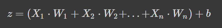
The formula above is the weighted average plus a bias term where, 

• z is the weighted sum of a neuron’s input
• Wn denotes the weights
• Xn denotes the independent variables, and
• b is the bias term.

If the formula looks familiar, that’s because it is linear regression. Without introducing non-linearity into the neurons, we would have linear regression, which is a simple model. The non-linear transformation allows our neural network to learn complex patterns. 

Activation functions

We’ve already alluded to some activation functions in the weight initialization section, but now you know their importance of them in a neural network architecture.

Let’s delve deeper into some common activation functions you’re likely to see when you read research papers and other people’s code.  

Sigmoid

The sigmoid function is characterized by an “S”-shaped curve that is bounded between the values zero and one. It’s a differentiable function, meaning the slope of the curve can be found at any two points, and monotonic, which means it’s neither entirely increasing nor decreasing. You would typically use the sigmoid activation function for binary classification problems.

Here’s how you can visualize your own sigmoid function using Python: 

# Sigmoid function in Python
import matplotlib.pyplot as plt
import numpy as np




x = np.linspace(-5, 5, 50)
z = 1/(1 + np.exp(-x))




plt.subplots(figsize=(8, 5))
plt.plot(x, z)
plt.grid()
plt.show()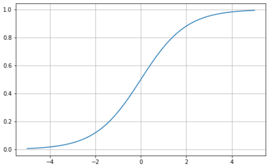

Tanh

The hyperbolic tangent (tanh) has the same “S”- shaped curve as the sigmoid function, except the values are bounded between -1 and 1. Thus, small inputs are mapped closer to -1, and larger inputs are mapped closer to 1.

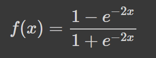
Here’s an example tanh function visualized using Python: 

# tanh function in Python
import matplotlib.pyplot as plt
import numpy as np




x = np.linspace(-5, 5, 50)
z = np.tanh(x)


plt.subplots(figsize=(8, 5))
plt.plot(x, z)
plt.grid()
plt.show()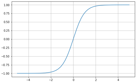

Softmax

The softmax function is generally used as an activation function in the output layer. It’s a generalization of the sigmoid function to multiple dimensions. Thus, it’s used in neural networks to predict class membership on more than two labels. 

Rectified Linear Unit (ReLU)

Using the sigmoid or tanh function to build deep neural networks is risky since they are more likely to suffer from the vanishing gradient problem. The rectified linear unit (ReLU) activation function came in as a solution to this problem and is often the default activation function for several neural networks. 

Here’s a visual example of the ReLU function using Python: 

# ReLU in Python
import matplotlib.pyplot as plt
import numpy as np


x = np.linspace(-5, 5, 50)
z = [max(0, i) for i in x]


plt.subplots(figsize=(8, 5))
plt.plot(x, z)
plt.grid()
plt.show()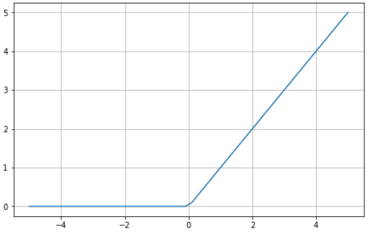

ReLU is bounded between zero and infinity: notice that for input values less than or equal to zero, the function returns zero, and for values above zero, the function returns the input value provided (i.e., if you input two the two will be returned). Ultimately, the ReLU function behaves extremely similar to a linear function, making it much easier to optimize and implement. 

The process from the input to the output layer is known as the forward pass or forward propagation. During this phase, the outputs generated by the model are used to compute a cost function to determine how the neural network is performing after each iteration. This information is then passed back through the model to correct the weights such that the model can make better predictions in a process known as backpropagation. 

Backpropagation

At the end of the first forward pass, the network makes predictions using the initialized weights, which are not tuned. Thus, it’s highly likely that the predictions the model makes will not be accurate. Using the loss calculated from forward propagation, we pass information back through the network to fine-tune the weights in a process known as backpropagation. 

Ultimately, we are using the optimization function to help us identify the weights that may reduce the error rate, making the model more reliable and increasing its ability to generalize to new instances. The mathematics for how this works is beyond the scope of this article, but the interested reader may learn more about backpropagation in our Introduction to Deep Learning in Python course.

PyTorch Tutorial: A step-by-step walkthrough of building a neural network from scratch

In this article section, we will build a simple artificial neural network model using the PyTorch library. Check out this DataCamp workspace to follow along with the code

PyTorch is one of the most popular libraries for deep learning. It provides a much more direct debugging experience than TensorFlow. It has several other perks such as distributed training, a robust ecosystem, cloud support, allowing you to write production-ready code, etc. You can learn more about PyTorch in the Introduction to Deep Learning with PyTorch skill track. 

Let’s get into the tutorial. 

Data definition & preparation 

The dataset we will be using in our tutorial is make_circles from scikit-learn – see the documentation. It’s a toy dataset containing a large circle with a smaller circle in a two-dimensional plane and two features. For our demonstration, we used 10,000 samples and added a 0.05 standard deviation of Gaussian noise to the data. 

Before we build our neural network, it’s good practice to split our data into training and testing sets so we can evaluate the model’s performance on unseen data.

import matplotlib.pyplot as plt
from sklearn.datasets import make_circles
from sklearn.model_selection import train_test_split

# Create a dataset with 10,000 samples.
X, y = make_circles(n_samples = 10000,
                    noise= 0.05,
                    random_state=26)

X_train, X_test, y_train, y_test = train_test_split(X, y, test_size=.33, random_state=26)

# Visualize the data.
fig, (train_ax, test_ax) = plt.subplots(ncols=2, sharex=True, sharey=True, figsize=(10, 5))
train_ax.scatter(X_train[:, 0], X_train[:, 1], c=y_train, cmap=plt.cm.Spectral)
train_ax.set_title("Training Data")
train_ax.set_xlabel("Feature #0")
train_ax.set_ylabel("Feature #1")

test_ax.scatter(X_test[:, 0], X_test[:, 1], c=y_test)
test_ax.set_xlabel("Feature #0")
test_ax.set_title("Testing data")
plt.show()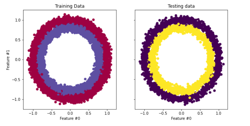

The next step is to convert the training and testing data from NumPy arrays to PyTorch tensors. To do this we are going to create a custom dataset for our training and test files. We are also going to leverage PyTorch’s Dataloader module so we can train our data in batches. Here’s the code: 

import warnings
warnings.filterwarnings("ignore")

!pip install torch -q

import torch
import numpy as np
from torch.utils.data import Dataset, DataLoader

# Convert data to torch tensors
class Data(Dataset):
    def __init__(self, X, y):
        self.X = torch.from_numpy(X.astype(np.float32))
        self.y = torch.from_numpy(y.astype(np.float32))
        self.len = self.X.shape[0]
       
    def __getitem__(self, index):
        return self.X[index], self.y[index]
   
    def __len__(self):
        return self.len
   
batch_size = 64

# Instantiate training and test data
train_data = Data(X_train, y_train)
train_dataloader = DataLoader(dataset=train_data, batch_size=batch_size, shuffle=True)

test_data = Data(X_test, y_test)
test_dataloader = DataLoader(dataset=test_data, batch_size=batch_size, shuffle=True)

# Check it's working
for batch, (X, y) in enumerate(train_dataloader):
    print(f"Batch: {batch+1}")
    print(f"X shape: {X.shape}")
    print(f"y shape: {y.shape}")
    break


"""
Batch: 1
X shape: torch.Size([64, 2])
y shape: torch.Size([64])
"""

Now let’s move on to implementing and training our neural network. 

Neural network implementation & model training

We are going to implement a simple two-layer neural network that uses the ReLU activation function (torch.nn.functional.relu). To do this we are going to create a class called NeuralNetwork that inherits from the nn.Module which is the base class for all neural network modules built in PyTorch. 

Here’s the code: 

import torch
from torch import nn
from torch import optim

input_dim = 2
hidden_dim = 10
output_dim = 1

class NeuralNetwork(nn.Module):
    def __init__(self, input_dim, hidden_dim, output_dim):
        super(NeuralNetwork, self).__init__()
        self.layer_1 = nn.Linear(input_dim, hidden_dim)
        nn.init.kaiming_uniform_(self.layer_1.weight, nonlinearity="relu")
        self.layer_2 = nn.Linear(hidden_dim, output_dim)
       
    def forward(self, x):
        x = torch.nn.functional.relu(self.layer_1(x))
        x = torch.nn.functional.sigmoid(self.layer_2(x))

        return x
       
model = NeuralNetwork(input_dim, hidden_dim, output_dim)
print(model)


"""
NeuralNetwork(
  (layer_1): Linear(in_features=2, out_features=10, bias=True)
  (layer_2): Linear(in_features=10, out_features=1, bias=True)
)
"""

And that’s all. 

To train the model we must define a loss function to use to calculate the gradients and an optimizer to update the parameters. For our demonstration, we are going to use binary crossentropy and stochastic gradient descent with a learning rate of 0.1. 

learning_rate = 0.1

loss_fn = nn.BCELoss()

optimizer = torch.optim.SGD(model.parameters(), lr=lea

Let’s train our model

num_epochs = 100
loss_values = []


for epoch in range(num_epochs):
    for X, y in train_dataloader:
        # zero the parameter gradients
        optimizer.zero_grad()
       
        # forward + backward + optimize
        pred = model(X)
        loss = loss_fn(pred, y.unsqueeze(-1))
        loss_values.append(loss.item())
        loss.backward()
        optimizer.step()

print("Training Complete")

"""
Training Complete
"""

Since we tracked the loss values, we can visualize the loss of the model over time. 

step = np.linspace(0, 100, 10500)

fig, ax = plt.subplots(figsize=(8,5))
plt.plot(step, np.array(loss_values))
plt.title("Step-wise Loss")
plt.xlabel("Epochs")
plt.ylabel("Loss")
plt.show()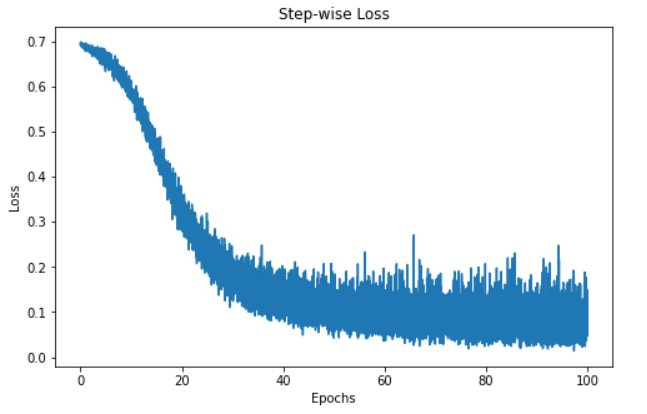

The visualization above shows the loss of our model over 100 epochs. Initially, the loss starts at 0.7 and gradually decreases – this informs us that our model has been improving its predictions over time. However, the model seems to plateau around the 60 epoch mark, which may be down to a variety of reasons, such as the model may be in the region of a local or global minimum of the loss function. 

Nonetheless, the model has been trained and is ready to make predictions on new instances – let’s look at how to do that in the next section.

Predictions & model evaluation

Making predictions with our PyTorch neural network is quite simple. 

"""
We're not training so we don't need to calculate the gradients for our outputs
"""
with torch.no_grad():
    for X, y in test_dataloader:
        outputs = model(X)
        predicted = np.where(outputs < 0.5, 0, 1)
        predicted = list(itertools.chain(*predicted))
        y_pred.append(predicted)
        y_test.append(y)
        total += y.size(0)
        correct += (predicted == y.numpy()).sum().item()

print(f'Accuracy of the network on the 3300 test instances: {100 * correct // total}%')

"""
Accuracy of the network on the 3300 test instances: 97%
"""

Note: Each run of the code would produce a different output so you may not get the same results. 

The code above loops through the test batches, which are stored in the test_dataloader variable, without calculating the gradients. We then predict the instances in the batch and store the results in a variable called outputs. Next, we determine set all the values less than 0.5 to 0 and those equal to or greater than 0.5 to 1. These values are then appended to a list for our predictions.

After that, we add the actual predictions of the instances in the batch to a variable named total. Then we calculate the number of correct predictions by identifying the number of predictions equal to the actual classes and totaling them. The total number of correct predictions for each batch is incremented and stored in our correct variable.

To calculate the accuracy of the overall model, we multiply the number of correct predictions by 100 (to get a percentage) and then divide it by the number of instances in our test set. Our model had 97% accuracy. We dig in further using the confusion matrix and scikit-learn’s classification_report to get a better understanding of how our model performed.

from sklearn.metrics import classification_report
from sklearn.metrics import confusion_matrix

import seaborn as sns


y_pred = list(itertools.chain(*y_pred))
y_test = list(itertools.chain(*y_test))


print(classification_report(y_test, y_pred))

"""
              precision    recall  f1-score   support

        0.0       0.98      0.97      0.98      1635
        1.0       0.98      0.98      0.98      1665

    accuracy                           0.98      3300
  macro avg       0.98      0.98      0.98      3300
weighted avg       0.98      0.98      0.98      3300

"""




cf_matrix = confusion_matrix(y_test, y_pred)

plt.subplots(figsize=(8, 5))

sns.heatmap(cf_matrix, annot=True, cbar=False, fmt="g")

plt.show()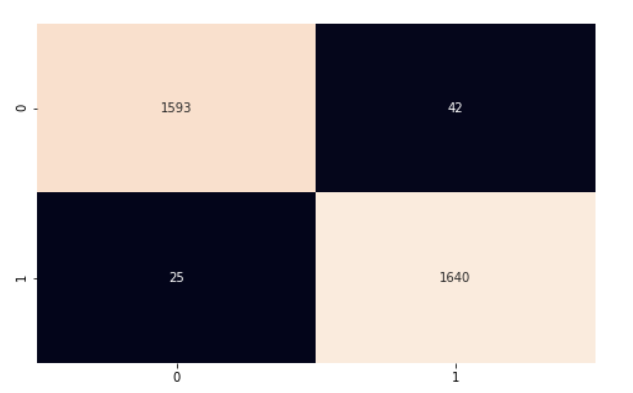

Our model is performing pretty well. I encourage you to explore the code and make some changes to help make what we’ve covered in this article stick.  

In this PyTorch tutorial, we covered the foundational basics of neural networks and used PyTorch, a Python library for deep learning, to implement our network. We used the circle’s dataset from scikit-learn to train a two-layer neural network for classification. We then made predictions on the data and evaluated our results using the accuracy metric.