Neural networks made easy

If you’ve dug into any articles on artificial intelligence, you’ve almost certainly run into the term “neural network.” Modeled loosely on the human brain, artificial neural networks enable computers to learn from being fed data.

The efficacy of this powerful branch of machine learning, more than anything else, has been responsible for ushering in a new era of artificial intelligence, ending a long-lived “AI Winter.” Simply put, the neural network may well be one of the most fundamentally disruptive technologies in existence today.

This guide to neural networks aims to give you a conversational level of understanding of deep learning. To this end, we’ll avoid delving into the math and instead rely as much as possible on analogies and animations.

Thinking by brute force

One of the early schools of AI taught that if you load up as much information as possible into a powerful computer and give it as many directions as possible to understand that data, it ought to be able to “think.” This was the idea behind chess computers like IBM’s famous Deep Blue: By exhaustively programming every possible chess move into a computer, as well as known strategies, and then giving it sufficient power, IBM programmers created a machine that, in theory, could calculate every possible move and outcome into the future and pick the sequence of subsequent moves to outplay its opponent. This actually works, as chess masters learned in 1997.*

With this sort of computing, the machine relies on fixed rules that have been painstakingly pre-programmed by engineers — if this happens, then that happens; if this happens, do this — and so it isn’t human-style flexible learning as we know it at all. It’s powerful supercomputing, for sure, but not “thinking” per se.

Teaching machines to learn

Over the past decade, scientists have resurrected an old concept that doesn’t rely on a massive encyclopedic memory bank, but instead on a simple and systematic way of analyzing input data that’s loosely modeled after human thinking. Known as deep learning, or neural networks, this technology has been around since the 1940s, but because of today’s exponential proliferation of data — images, videos, voice searches, browsing habits and more — along with supercharged and affordable processors, it is at last able to begin to fulfill its true potential.

Machines — they’re just like us!

An artificial (as opposed to human) neural network (ANN) is an algorithmic construct that enables machines to learn everything from voice commands and playlist curation to music composition and image recognition.The typical ANN consists of thousands of interconnected artificial neurons, which are stacked sequentially in rows that are known as layers, forming millions of connections. In many cases, layers are only interconnected with the layer of neurons before and after them via inputs and outputs. (This is quite different from neurons in a human brain, which are interconnected every which way.)

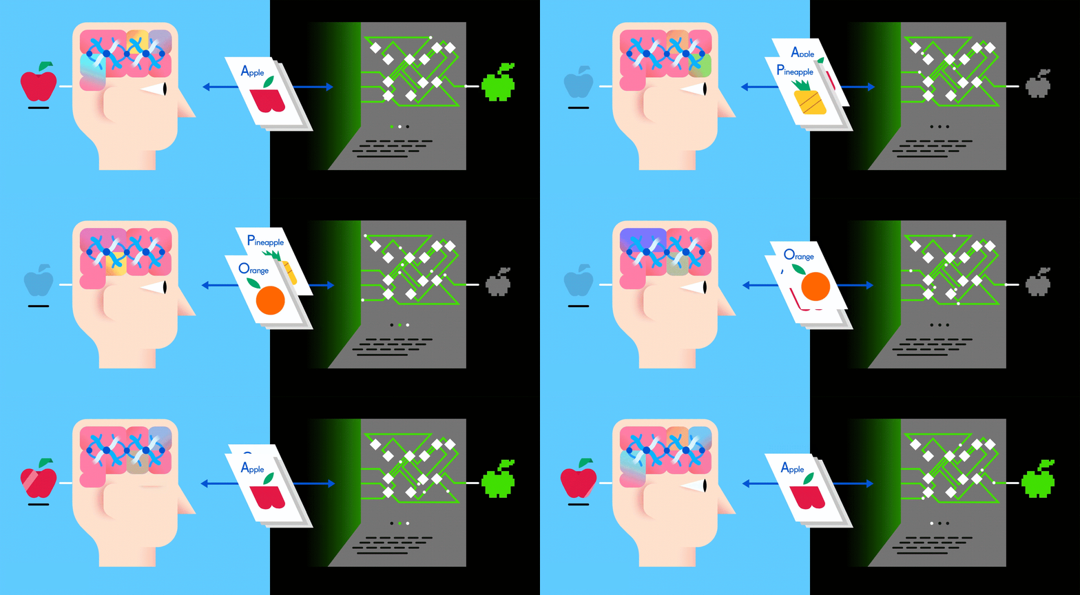
This layered ANN is one of the main ways to go about machine learning today, and feeding it vast amounts of labeled data enables it to learn how to interpret that data like (and sometimes better than) a human.

Just as when parents teach their kids to identify apples and oranges in real life, for computers too, practice makes perfect.

Take, for example, image recognition, which relies on a particular type of neural network known as the convolutional neural network (CNN) — so called because it uses a mathematical process known as convolution to be able to analyze images in non-literal ways, such as identifying a partially obscured object or one that is viewable only from certain angles. (There are other types of neural networks, including recurrent neural networks and feed-forward neural networks, but these are less useful for identifying things like images, which is the example we’re going to use below.)

All aboard the network training

So how do neural networks learn? Let’s look at a very simple, yet effective, procedure called supervised learning. Here, we feed the neural network vast amounts of training data, labeled by humans so that a neural network can essentially fact-check itself as it’s learning.

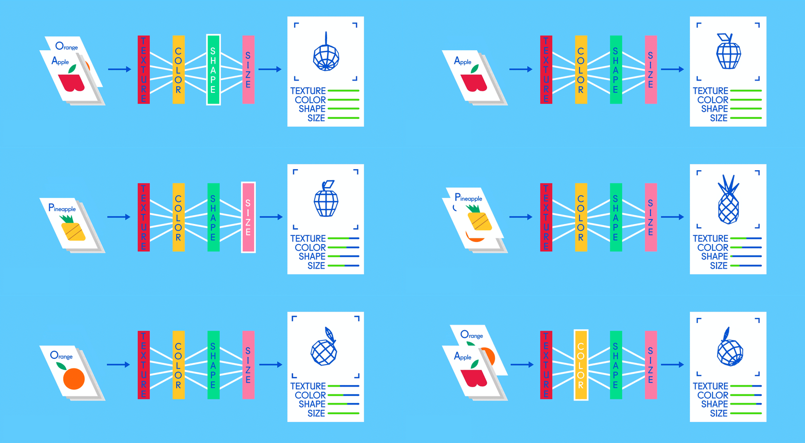
Let’s say this labeled data consists of pictures of apples and oranges, respectively. The pictures are the data; “apple” and “orange” are the labels, depending on the picture. As pictures are fed in, the network breaks them down into their most basic components, i.e. edges, textures and shapes. As the picture propagates through the network, these basic components are combined to form more abstract concepts, i.e. curves and different colors which, when combined further, start to look like a stem, an entire orange, or both green and red apples.

At the end of this process, the network attempts to make a prediction as to what’s in the picture. At first, these predictions will appear as random guesses, as no real learning has taken place yet. If the input image is an apple, but “orange” is predicted, the network’s inner layers will need to be adjusted.

The adjustments are carried out through a process called backpropagation to increase the likelihood of predicting “apple” for that same image the next time around. This happens over and over until the predictions are more or less accurate and don’t seem to be improving. Just as when parents teach their kids to identify apples and oranges in real life, for computers too, practice makes perfect. If, in your head, you just thought “hey, that sounds like learning,” then you may have a career in AI.

So many layers…

Typically, a convolutional neural network has four essential layers of neurons besides the input and output layers:

• Convolution

• Activation

• Pooling

• Fully connected

Convolution

In the initial convolution layer or layers, thousands of neurons act as the first set of filters, scouring every part and pixel in the image, looking for patterns. As more and more images are processed, each neuron gradually learns to filter for specific features, which improves accuracy.

In the case of apples, one filter might be focused on finding the color red, while another might be looking for rounded edges and yet another might be identifying thin, stick-like stems. If you’ve ever had to clean out a cluttered basement to prepare for a garage sale or a big move — or worked with a professional organizer — then you know what it is to go through everything and sort it into different-themed piles (books, toys, electronics, objets d’art, clothes). That’s sort of what a convolutional layer does with an image by breaking it down into different features.

One advantage of neural networks is that they are capable of learning in a nonlinear way.

What’s particularly powerful — and one of the neural network’s main claims to fame — is that unlike earlier AI methods (Deep Blue and its ilk), these filters aren’t hand designed; they learn and refine themselves purely by looking at data.

The convolution layer essentially creates maps — different, broken-down versions of the picture, each dedicated to a different filtered feature — that indicate where its neurons see an instance (however partial) of the color red, stems, curves and the various other elements of, in this case, an apple. But because the convolution layer is fairly liberal in its identifying of features, it needs an extra set of eyes to make sure nothing of value is missed as a picture moves through the network.

Activation

One advantage of neural networks is that they are capable of learning in a nonlinear way, which, in mathless terms, means they are able to spot features in images that aren’t quite as obvious — pictures of apples on trees, some of them under direct sunlight and others in the shade, or piled into a bowl on a kitchen counter. This is all thanks to the activation layer, which serves to more or less highlight the valuable stuff — both the straightforward and harder-to-spot varieties.

In the world of our garage-sale organizer or clutter consultant, imagine that from each of those separated piles of things we’ve cherry-picked a few items — a handful of rare books, some classic t-shirts from our college days to wear ironically — that we might want to keep. We stick these “maybe” items on top of their respective category piles for another consideration later.

Pooling

All this “convolving” across an entire image generates a lot of information, and this can quickly become a computational nightmare. Enter the pooling layer, which shrinks it all into a more general and digestible form. There are many ways to go about this, but one of the most popular is “max pooling,” which edits down each feature map into a Reader’s Digest version of itself, so that only the best examples of redness, stem-ness or curviness are featured.

In the garage spring cleaning example, if we were using famed Japanese clutter consultant Marie Kondo’s principles, our pack rat would have to choose only the things that “spark joy” from the smaller assortment of favorites in each category pile, and sell or toss everything else. So now we still have all our piles categorized by type of item, but only consisting of the items we actually want to keep; everything else gets sold. (And this, by the way, ends our de-cluttering analogy to help describe the filtering and downsizing that goes on inside a neural network.)

At this point, a neural network designer can stack subsequent layered configurations of this sort — convolution, activation, pooling — and continue to filter down images to get higher-level information. In the case of identifying an apple in pictures, the images get filtered down over and over, with initial layers showing just barely discernable parts of an edge, a blip of red or just the tip of a stem, while subsequent, more filtered layers will show entire apples. Either way, when it’s time to start getting results, the fully connected layer comes into play.

Fully connected

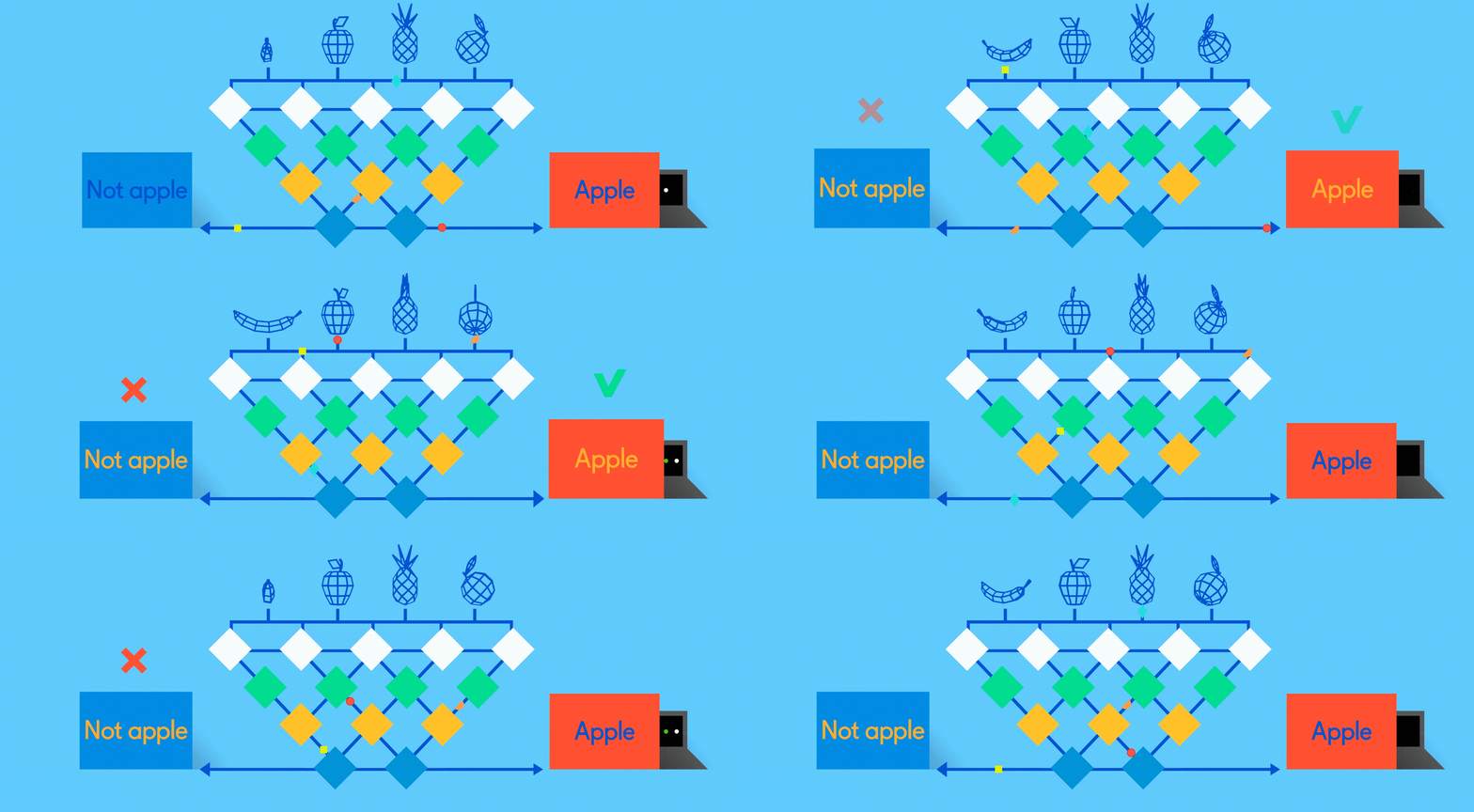
Now it’s time to start getting answers. In the fully connected layer, each reduced, or “pooled,” feature map is “fully connected” to output nodes (neurons) that represent the items the neural network is learning to identify. If the network is tasked with learning how to spot cats, dogs, guinea pigs and gerbils, then it’ll have four output nodes. In the case of the neural network we’ve been describing, it’ll just have two output nodes: one for “apples” and one for “oranges.”

If the picture that has been fed through the network is of an apple, and the network has already undergone some training and is getting better with its predictions, then it’s likely that a good chunk of the feature maps contain quality instances of apple features. This is where these final output nodes start to fulfill their destiny, with a reverse election of sorts.

Tweaks and adjustments are made to help each neuron better identify the data at every level.

The job (which they’ve learned “on the job”) of both the apple and orange nodes is essentially to “vote” for the feature maps that contain their respective fruits. So, the more the “apple” node thinks a particular feature map contains “apple” features, the more votes it sends to that feature map. Both nodes have to vote on every single feature map, regardless of what it contains. So in this case, the “orange” node won’t send many votes to any of the feature maps, because they don’t really contain any “orange” features. In the end, the node that has sent the most votes out — in this example, the “apple” node — can be considered the network’s “answer,” though it’s not quite that simple.

Because the same network is looking for two different things — apples and oranges — the final output of the network is expressed as percentages. In this case, we’re assuming that the network is already a bit down the road in its training, so the predictions here might be, say, 75 percent “apple” and 25 percent “orange.” Or, if it’s earlier in the training, it might be more inaccurate and determine that it’s 20 percent “apple” and 80 percent “orange.” Oops.

If at first you don’t succeed, try, try, try again

So, in its early stages, the neural network spits out a bunch of wrong answers in the form of percentages. The 20 percent “apple” and 80 percent “orange” prediction is clearly wrong, but since this is supervised learning with labeled training data, the network is able to figure out where and how that error occurred through a system of checks and balances known as backpropagation.

Now, this is a mathless explanation, so suffice it to say that backpropagation sends feedback to the previous layer’s nodes about just how far off the answers were. That layer then sends the feedback to the previous layer, and on and on like a game of telephone until it’s back at convolution. Tweaks and adjustments are made to help each neuron better identify the data at every level when subsequent images go through the network.

This process is repeated over and over until the neural network is identifying apples and oranges in images with increasing accuracy, eventually ending up at 100 percent correct predictions — though many engineers consider 85 percent to be acceptable. And when that happens, the neural network is ready for prime time and can start identifying apples in pictures professionally.

*This is different than Google’s AlphaGo which used a self-learned neural net to evaluate board positions and ultimately beat a human at Go, versus Deep Blue, which used a hard-coded function written by a human.