Neural Network Algorithms | 4 Types of Neural Network Alogrithms

Neural Network Algorithms

Mục Lục

Introduction to Neural Network Algorithms

The following article provides an outline for Neural Network Algorithms. Let’s first know what does a Neural Network mean? Neural networks are inspired by the biological neural networks in the brain, or we can say the nervous system. It has generated a lot of excitement, and research is still going on this subset of Machine Learning in the industry. The basic computational unit of a neural network is a neuron or node. It receives values from other neurons and computes the output. Each node/neuron is associated with weight(w). This weight is given as per the relative importance of that particular neuron or node.

So, if we take f as the node function, then the node function f will provide output as shown below:

Start Your Free Data Science Course

Hadoop, Data Science, Statistics & others

Output of neuron(Y) = f(w1.X1 +w2.X2 +b)

Where w1 and w2 are weight, X1 and X2 are numerical inputs, whereas b is the bias.
The above function f is a non-linear function also called the activation function. Its basic purpose is to introduce non-linearity as almost all real-world data is non-linear, and we want neurons to learn these representations.

Different Neural Network Algorithms

Given below are the four different algorithms:

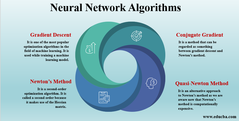
1. Gradient Descent

It is one of the most popular optimization algorithms in the field of machine learning. It is used while training a machine learning model. In simple words, It is basically used to find values of the coefficients that simply reduce the cost function as much as possible. First of all, we start by defining some parameter values, and then by using calculus, we start to iteratively adjust the values so that the lost function is reduced.

Now, let’s come to the part of what is gradient?. So, a gradient means by much the output of any function will change if we decrease the input by little or in other words, we can call it to the slope. If the slope is steep, the model will learn faster similarly; a model stops learning when the slope is zero. This is because it is a minimization algorithm that minimizes a given algorithm.

Below the formula for finding the next position is shown in the case of gradient descent.

Where b is the next position,

a is the current position; gamma is awaiting function.

So, as you can see, gradient descent is a very sound technique, but there are many areas where gradient descent does not work properly.

Below some of them are provided:

If the algorithm is not executed properly then we may encounter something like the problem of vanishing gradient. These occur when the gradient is too small or too large.
Problems come when data arrangement poses a non-convex optimization problem. Gradient descent works only with problems which are the convex optimized problem.
One of the very important factors to look for while applying this algorithm is resources. If we have less memory assigned for the application, We should avoid gradient descent algorithm.

2. Newton’s Method

It is a second-order optimization algorithm. It is called a second-order because it makes use of the Hessian matrix. So, the Hessian matrix is nothing but a squared matrix of second-order partial derivatives of a scalar-valued function. In Newton’s method optimization algorithm, It is applied to the first derivative of a double differentiable function f so that it can find the roots/stationary points. Let’s now get into the steps required by Newton’s method for optimization.

It first evaluates the loss index. It then checks whether the stopping criteria is true or false. If false, it then calculates Newton’s training direction and the training rate and then improves the parameters or weights of the neuron, and again the same cycle continues. So, you can now say that it takes fewer steps as compared to gradient descent to get the minimum value of the function. Though it takes fewer steps as compared to the gradient descent algorithm still it is not used widely as the exact calculation of hessian and its inverse are computationally very expensive.

3. Conjugate Gradient

It is a method that can be regarded as something between gradient descent and Newton’s method. The main difference is that it accelerates the slow convergence, which we generally associate with gradient descent. Another important fact is that it can be used for both linear as well as non-linear systems, and it is an iterative algorithm.

It was developed by Magnus Hestenes and Eduard Stiefel. As already mentioned above that it produces faster convergence than gradient descent; the reason it is able to do it is that in the Conjugate Gradient algorithm, the search is done along with the conjugate directions, due to which it converges faster than gradient descent algorithms. One important point to note is that γ is called the conjugate parameter.

The training direction is periodically reset to the negative of the gradient. This method is more effective than gradient descent in training the neural network as it does not require the Hessian matrix, which increases the computational load, and it also convergences faster than gradient descent. It is appropriate to use in large neural networks.

4. Quasi-Newton Method

It is an alternative approach to Newton’s method as we are aware now that Newton’s method is computationally expensive. This method solves those drawbacks to an extent such that instead of calculating the Hessian matrix and then calculating the inverse directly, this method builds up an approximation to inverse Hessian at each iteration of this algorithm.

Now, this approximation is calculated using the information from the first derivative of the loss function. So, we can say that it is probably the best-suited method to deal with large networks as it saves computation time, and also, it is much faster than gradient descent or conjugate gradient method.

Conclusion

Let’s compare the computational speed and memory for the above-mentioned algorithms. As per memory requirements, gradient descent requires the least memory, and it is also the slowest. On the contrary to that Newton’s method requires more computational power. So taking all these into consideration, the Quasi-Newton method is the best suited.