Introduction To Tensorflow | Deep Learning Using Tensorflow

Overview

• Learn how to implement neural networks using TensorFlow
• Understand the applications of neural networks with the help of a practice problem

Introduction

If you have been following Data Science / Machine Learning, you just can’t miss the buzz around Deep Learning and Neural Networks. Organizations are looking for people with Deep Learning skills wherever they can. From running competitions to open sourcing projects and paying big bonuses, people are trying every possible thing to tap into this limited pool of talent.

Self driving engineers are being hunted by the big guns in automobile industry, as the industry stands on the brink of biggest disruption it faced in last few decades!

If you are excited by the prospects deep learning has to offer, but have not started your journey yet – I am here to enable it. Starting with this article, I will write a series of articles on deep learning covering the popular Deep Learning libraries and their hands-on implementation.

In this article, I will introduce TensorFlow to you. After reading this article you will be able to understand application of neural networks and use TensorFlow to solve a real life problem. This article will require you to know the basics of neural networks and have familiarity with programming. Although the code in this article is in python, I have focused on the concepts and stayed as language-agnostic as possible.

Let’s get started!

Table of Contents

• When to apply neural nets?
• General way to solve problems with Neural Networks
• Understanding Image data and popular libraries to solve it
• What is TensorFlow?
• A typical “flow” of TensorFlow
• Implementing MLP in TensorFlow
• Limitations of TensorFlow
• TensorFlow vs. other libraries
• Where to go from here?

When to apply Neural Networks ?

Neural Networks have been in the spotlight for quite some time now. For a more detailed explanation on neural network and deep learning read here. Its “deeper” versions are making tremendous breakthroughs in many fields such as image recognition, speech and natural language processing etc.

The main question that arises is when to and when not to apply neural networks? This field is like a gold mine right now, with many discoveries uncovered everyday. And to be a part of this “gold rush”, you have to keep a few things in mind:

• Firstly, neural networks require clear and informative data (and mostly big data) to train. Try to imagine Neural Networks as a child. It first observes how its parent walks. Then it tries to walk on its own, and with its every step, the child learns how to perform a particular task. It may fall a few times, but after few unsuccessful attempts, it learns how to walk. If you don’t let it walk, it might not ever learn how to walk. The more exposure you can provide to the child, the better it is.
• It is prudent to use Neural Networks for complex problems such as image processing. Neural nets belong to a class of algorithms called representation learning algorithms. These algorithms break down complex problems into simpler form so that they become understandable (or “representable”). Think of it as chewing food before you gulp. This would be harder for traditional (non-representation learning) algorithms.
• When you have appropriate type of neural network to solve the problem. Each problem has its own twists. So the data decides the way you solve the problem. For example, if the problem is of sequence generation, recurrent neural networks are more suitable. Whereas, if it is image related problem, you would probably be better of taking convolutional neural networks for a change.
• Last but not the least, hardware requirements are essential for running a deep neural network model. Neural nets were “discovered” long ago, but they are shining in the recent years for the main reason that computational resources are better and more powerful. If you want to solve a real life problem with these networks, get ready to buy some high-end hardware!

General way to solve problems with Neural Networks

Neural networks is a special type of machine learning (ML) algorithm. So as every ML algorithm, it follows the usual ML workflow of data preprocessing, model building and model evaluation. For the sake of conciseness, I have listed out a TO DO list of how to approach a Neural Network problem.

• Check if it is a problem where Neural Network gives you uplift over traditional algorithms (refer to the checklist in the section above)
• Do a survey of which Neural Network architecture is most suitable for the required problem
• Define Neural Network architecture through which ever language / library you choose.
• Convert data to right format and divide it in batches
• Pre-process the data according to your needs
• Augment Data to increase size and make better trained models
• Feed batches to Neural Network
• Train and monitor changes in training and validation data sets
• Test your model, and save it for future use

For this article, I will be focusing on image data. So let us understand that first before we delve into TensorFlow.

Understanding Image data and popular libraries to solve it

Images are mostly arranged as 3-D arrays, with the dimensions referring to height, width and color channel. For example, if you take a screenshot of your PC at this moment, it would be first convert into a 3-D array and then compress it  ‘.jpeg’ or ‘.png’ file formats.

While these images are pretty easy to understand to a human, a computer has a hard time to understand them. This phenomenon is called “Semantic gap”. Our brain can look at the image and understand the complete picture in a few seconds. On the other hand, computer sees image as just an array of numbers. So the problem is how to we explain this image to the machine?

In early days, people tried to break down the image into “understandable” format for the machine like a “template”. For example, a face always has a specific structure which is somewhat preserved in every human, such as the position of eyes, nose or the shape of our face. But this method would be tedious, because when the number of objects to recognise would increase, the “templates” would not hold.

Fast forward to 2012, a deep neural network architecture won the ImageNet challenge, a prestigious challenge to recognise objects from natural scenes. It continued to reign its sovereignty in all the upcoming ImageNet challenges, thus proving the usefulness to solve image problems.

So which library / language do people normally use to solve image recognition problems? One recent survey I did that most of the popular deep learning libraries have interface for Python, followed by Lua, Java and Matlab. The most popular libraries, to name a few, are:

Now, that  you understand how an image is stored and which are the common libraries used, let us look at what TensorFlow has to offer.

What is TensorFlow?

Lets start with the official definition,

“TensorFlow is an open source software library for numerical computation using dataflow graphs. Nodes in the graph represents mathematical operations, while graph edges represent multi-dimensional data arrays (aka tensors) communicated between them. The flexible architecture allows you to deploy computation to one or more CPUs or GPUs in a desktop, server, or mobile device with a single API.”

If that sounds a bit scary – don’t worry. Here is my simple definition – look at TensorFlow as nothing but numpy with a twist. If you have worked on numpy before, understanding TensorFlow will be a piece of cake! A major difference between numpy and TensorFlow is that TensorFlow follows a lazy programming paradigm. It first builds a graph of all the operation to be done, and then when a “session” is called, it “runs” the graph. It’s built to be scalable, by changing internal data representation to tensors (aka multi-dimensional arrays). Building a computational graph can be considered as the main ingredient of TensorFlow. To know more about mathematical constitution of a computational graph, read this article.

It’s easy to classify TensorFlow as a neural network library, but it’s not just that. Yes, it was designed to be a powerful neural network library. But it has the power to do much more than that. You can build other machine learning algorithms on it such as decision trees or k-Nearest Neighbors. You can literally do everything you normally would do in numpy! It’s aptly called “numpy on steroids”

The advantages of using TensorFlow are:

• It has an intuitive construct, because as the name suggests it has “flow of tensors”. You can easily visualize each and every part of the graph.
• Easily train on cpu/gpu for distributed computing
• Platform flexibility. You can run the models wherever you want, whether it is on mobile, server or PC.

A typical “flow” of TensorFlow

Every library has its own “implementation details”, i.e. a way to write which follows its coding paradigm. For example, when implementing scikit-learn, you first create object of the desired algorithm, then build a model on train and get predictions on test set, something like this:

# define hyperparamters of ML algorithm
clf
 
=
 
svm
.
SVC
(
gamma
=
0.001
,
 
C
=
100.
)
# train 
clf
.
fit
(
X
,
 
y
)
# test 
clf
.
predict
(
X_test
)

As I said earlier, TensorFlow follows a lazy approach. The usual workflow of running a program in TensorFlow is as follows:

• Build a computational graph, this can be any mathematical operation TensorFlow supports.
• Initialize variables, to compile the variables defined previously
  
• Create session, this is where the magic starts!
  
• Run graph in session, the compiled graph is passed to the session, which starts its execution.
  
• Close session, shutdown the session.

Few terminologies used in TensoFlow;

• placeholder: A way to feed data into the graphs

• feed_dict: A dictionary to pass numeric values to computational graph

Lets write a small program to add two numbers!

# import tensorflow
import tensorflow as tf

# build computational graph
a
 
=
 
tf
.
placeholder
(
tf
.
int16
)
b
 
=
 
tf
.
placeholder
(
tf
.
int16
)

addition
 
=
 
tf
.
add
(
a
,
 
b
)

# initialize variables
init = tf.initialize_all_variables()

# create session and run the graph
with
 
tf
.
Session
()
 
as
 
sess
:
    sess.run(init)
    
print
 
"Addition: 
%i
"
 
%
 
sess
.
run
(
addition
,
 
feed_dict
=
{
a
:
 
2
,
 
b
:
 
3
})

# close session
sess.close()

Implementing Neural Network in TensorFlow

Note: We could have used a different neural network architecture to solve this problem, but for the sake of simplicity, we settle on feed forward multilayer perceptron with an in depth implementation.

Let us remember what we learned about neural networks first.

A typical implementation of Neural Network would be as follows:

• Define Neural Network architecture to be compiled
• Transfer data to your model
• Under the hood, the data is first divided into batches, so that it can be ingested. The batches are first preprocessed, augmented and then fed into Neural Network for training
• The model then gets trained incrementally
• Display the accuracy for a specific number of timesteps
• After training save the model for future use
• Test the model on a new data and check how it performs

Here we solve our deep learning practice problem – Identify the Digits.  Let’s for a moment take a look at our problem statement.

Our problem is an image recognition, to identify digits from a given 28 x 28 image. We have a subset of images for training and the rest for testing our model. So first, download the train and test files. The dataset contains a zipped file of all the images in the dataset and both the train.csv and test.csv have the name of corresponding train and test images. Any additional features are not provided in the datasets, just the raw images are provided in ‘.png’ format.

As you know we will use TensorFlow to make a neural network model. So you should first install TensorFlow in your system. Refer the official installation guide for installation, as per your system specifications.

We will follow the template as described above. Create a Jupyter notebook with python 2.7 kernel and follow the steps below.

• Let’s import all the required modules

%pylab inline

import os
import numpy as np
import pandas as pd
from scipy.misc import imread
from sklearn.metrics import accuracy_score
import tensorflow as tf

• Let’s set a seed value, so that we can control our models randomness

# To stop potential randomness
seed = 128
rng = np.random.RandomState(seed)

• The first step is to set directory paths, for safekeeping!

root_dir = os.path.abspath('../..')
data_dir = os.path.join(root_dir, 'data')
sub_dir = os.path.join(root_dir, 'sub')

# check for existence
os.path.exists(root_dir)
os.path.exists(data_dir)
os.path.exists(sub_dir)

• Now let us read our datasets. These are in .csv formats, and have a filename along with the appropriate labels

train = pd.read_csv(os.path.join(data_dir, 'Train', 'train.csv'))
test = pd.read_csv(os.path.join(data_dir, 'Test.csv'))

sample_submission = pd.read_csv(os.path.join(data_dir, 'Sample_Submission.csv'))

train.head()

filename
label

0
0.png
4

1
1.png
9

2
2.png
1

3
3.png
7

4
4.png
3

• Let us see what our data looks like! We read our image and display it.

img_name = rng.choice(train.filename)
filepath = os.path.join(data_dir, 'Train', 'Images', 'train', img_name)

img = imread(filepath, flatten=True)

pylab.imshow(img, cmap='gray')
pylab.axis('off')
pylab.show()

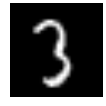
The above image is represented as numpy array, as seen below

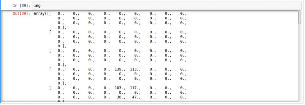
• For easier data manipulation, let’s store all our images as numpy arrays

temp = []
for img_name in train.filename:
    image_path = os.path.join(data_dir, 'Train', 'Images', 'train', img_name)
    img = imread(image_path, flatten=True)
    img = img.astype('float32')
    temp.append(img)
    
train_x = np.stack(temp)

temp = []
for img_name in test.filename:
    image_path = os.path.join(data_dir, 'Train', 'Images', 'test', img_name)
    img = imread(image_path, flatten=True)
    img = img.astype('float32')
    temp.append(img)
    
test_x = np.stack(temp)

• As this is a typical ML problem, to test the proper functioning of our model we create a validation set. Let’s take a split size of 70:30 for train set vs validation set

split_size = int(train_x.shape[0]*0.7)

train_x, val_x = train_x[:split_size], train_x[split_size:]
train_y, val_y = train.label.values[:split_size], train.label.values[split_size:]

• Now we define some helper functions, which we use later on, in our programs

def dense_to_one_hot(labels_dense, num_classes=10):
    """Convert class labels from scalars to one-hot vectors"""
    num_labels = labels_dense.shape[0]
    index_offset = np.arange(num_labels) * num_classes
    labels_one_hot = np.zeros((num_labels, num_classes))
    labels_one_hot.flat[index_offset + labels_dense.ravel()] = 1
    
    return labels_one_hot

def preproc(unclean_batch_x):
    """Convert values to range 0-1"""
    temp_batch = unclean_batch_x / unclean_batch_x.max()
    
    return temp_batch

def batch_creator(batch_size, dataset_length, dataset_name):
    """Create batch with random samples and return appropriate format"""
    batch_mask = rng.choice(dataset_length, batch_size)
    
    batch_x = eval(dataset_name + '_x')[[batch_mask]].reshape(-1, input_num_units)
    batch_x = preproc(batch_x)
    
    if dataset_name == 'train':
        batch_y = eval(dataset_name).ix[batch_mask, 'label'].values
        batch_y = dense_to_one_hot(batch_y)
        
    return batch_x, batch_y

• Now comes the main part! Let us define our neural network architecture. We define a neural network with 3 layers;  input, hidden and output. The number of neurons in input and output are fixed, as the input is our 28 x 28 image and the output is a 10 x 1 vector representing the class. We take 500 neurons in the hidden layer. This number can vary according to your need. We also assign values to remaining variables. Read the article on fundamentals of neural network to know more in depth of how it works.

### set all variables

# number of neurons in each layer
input_num_units = 28*28
hidden_num_units = 500
output_num_units = 10

# define placeholders
x = tf.placeholder(tf.float32, [None, input_num_units])
y = tf.placeholder(tf.float32, [None, output_num_units])

# set remaining variables
epochs = 5
batch_size = 128
learning_rate = 0.01

### define weights and biases of the neural network (refer this article if you don't understand the terminologies)

weights = {
    'hidden': tf.Variable(tf.random_normal([input_num_units, hidden_num_units], seed=seed)),
    'output': tf.Variable(tf.random_normal([hidden_num_units, output_num_units], seed=seed))
}

biases = {
    'hidden': tf.Variable(tf.random_normal([hidden_num_units], seed=seed)),
    'output': tf.Variable(tf.random_normal([output_num_units], seed=seed))
}

• Now create our neural networks computational graph

hidden_layer = tf.add(tf.matmul(x, weights['hidden']), biases['hidden'])
hidden_layer = tf.nn.relu(hidden_layer)

output_layer = tf.matmul(hidden_layer, weights['output']) + biases['output']

• Also, we need to define cost of our neural network

cost = tf.reduce_mean(tf.nn.softmax_cross_entropy_with_logits(output_layer, y))

• And set the optimizer, i.e. our backpropogation algorithm. Here we use Adam, which is an efficient variant of Gradient Descent algorithm. There are a number of other optimizers available in tensorflow (refer here)

optimizer = tf.train.AdamOptimizer(learning_rate=learning_rate).minimize(cost)

• After defining our neural network architecture, let’s initialize all the variables

init = tf.initialize_all_variables()

• Now let us create a session, and run our neural network in the session. We also validate our models accuracy on validation set that we created

with tf.Session() as sess:
    # create initialized variables
    sess.run(init)
    
    ### for each epoch, do:
    ###   for each batch, do:
    ###     create pre-processed batch
    ###     run optimizer by feeding batch
    ###     find cost and reiterate to minimize
    
    for epoch in range(epochs):
        avg_cost = 0
        total_batch = int(train.shape[0]/batch_size)
        for i in range(total_batch):
            batch_x, batch_y = batch_creator(batch_size, train_x.shape[0], 'train')
            _, c = sess.run([optimizer, cost], feed_dict = {x: batch_x, y: batch_y})
            
            avg_cost += c / total_batch
            
        print "Epoch:", (epoch+1), "cost =", "{:.5f}".format(avg_cost)
    
    print "\nTraining complete!"
    
    
    # find predictions on val set
    pred_temp = tf.equal(tf.argmax(output_layer, 1), tf.argmax(y, 1))
    accuracy = tf.reduce_mean(tf.cast(pred_temp, "float"))
    print "Validation Accuracy:", accuracy.eval({x: val_x.reshape(-1, input_num_units), y: dense_to_one_hot(val_y)})
    
    predict = tf.argmax(output_layer, 1)
    pred = predict.eval({x: test_x.reshape(-1, input_num_units)})

This will be the output of the above code

Epoch: 1 cost = 8.93566
Epoch: 2 cost = 1.82103
Epoch: 3 cost = 0.98648
Epoch: 4 cost = 0.57141
Epoch: 5 cost = 0.44550

Training complete!
Validation Accuracy: 0.952823

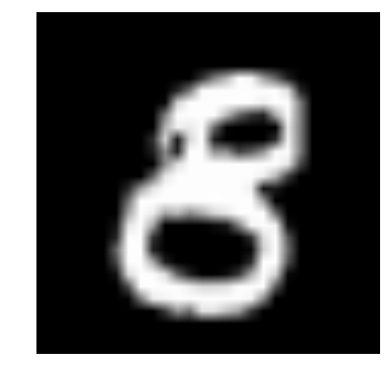
• To test our model with our own eyes, let’s visualize its predictions

img_name = rng.choice(test.filename)
filepath = os.path.join(data_dir, 'Train', 'Images', 'test', img_name)

img = imread(filepath, flatten=True)

test_index = int(img_name.split('.')[0]) - 49000

print "Prediction is: ", pred[test_index]

pylab.imshow(img, cmap='gray')
pylab.axis('off')
pylab.show()

Prediction is:  8

• We see that our model performance is pretty good! Now let’s create a submission

sample_submission.filename = test.filename

 sample_submission.label = pred

sample_submission.to_csv(os.path.join(sub_dir, 'sub01.csv'), index=False)

And done! We just created our own trained neural network!

Limitations of TensorFlow

• Even though TensorFlow is powerful, it’s still a low level library. For example, it can be considered as a machine level language. But for most of the purpose, you need modularity and high level interface such as keras
• It’s still in development, so much more awesomeness to come!
• It depends on your hardware specs, the more the merrier
• Still not an API for many languages.
• There are still many things yet to be included in TensorFlow, such as OpenCL support.

Most of the above mentioned are in the sights of TensorFlow developers. They have made a roadmap for specifying how the library should be developed in the future.

TensorFlow vs. Other Libraries

TensorFlow is built on similar principles as Theano and Torch of using mathematical computational graphs. But with the additional support of distributed computing, TensorFlow comes out to be better at solving complex problems. Also deployment of TensorFlow models is already supported which makes it easier to use for industrial purposes, giving a fight to commercial libraries such as Deeplearning4j, H2O and Turi. TensorFlow has APIs for Python, C++ and Matlab. There’s also a recent surge for support for other languages such as Ruby and R. So, TensorFlow is trying to have a universal language support.

Where to go from here?

So you saw how to build a simple neural network with TensorFlow. This code is meant for people to understand how to get started implementing TensorFlow, so take it with a pinch of salt. Remember that to solve more complex real life problems, you have to tweak the code a little bit.

Many of the above functions can be abstracted to give a seamless end-to-end workflow. If you have worked with scikit-learn, you might know how a high level library abstracts “under the hood” implementations to give end-users a more easier interface. Although TensorFlow has most of the implementations already abstracted, high level libraries are emerging such as TF-slim and TFlearn.

Useful Resources

End Notes

I hope you found this article helpful. Now, it’s time for you to practice and read as much as you can. Good luck! If you follow a different approach / package / library to get started with Neural Networks, I’d love to interact with you in comments. If you have any more suggestions, drop in your comments below. And to gain expertise in working in neural network don’t forget to try out our deep learning practice problem – Identify the Digits.

You can test your skills and knowledge. Check out Live Competitions and compete with best Data Scientists from all over the world.

Related