Implementing the Perceptron Neural Network with Python - PyImageSearch

First introduced by Rosenblatt in 1958, The Perceptron: A Probabilistic Model for Information Storage and Organization in the Brain is arguably the oldest and most simple of the ANN algorithms. Following this publication, Perceptron-based techniques were all the rage in the neural network community. This paper alone is hugely responsible for the popularity and utility of neural networks today.

But then, in 1969, an “AI Winter” descended on the machine learning community that almost froze out neural networks for good. Minsky and Papert published Perceptrons: an introduction to computational geometry, a book that effectively stagnated research in neural networks for almost a decade — there is much controversy regarding the book (Olazaran, 1996), but the authors did successfully demonstrate that a single layer Perceptron is unable to separate nonlinear data points.

Given that most real-world datasets are naturally nonlinearly separable, this it seemed that the Perceptron, along with the rest of neural network research, might reach an untimely end.

Between the Minsky and Papert publication and the broken promises of neural networks revolutionizing industry, the interest in neural networks dwindled substantially. It wasn’t until we started exploring deeper networks (sometimes called multi-layer perceptrons) along with the backpropagation algorithm (Werbos and Rumelhart et al.) that the “AI Winter” in the 1970s ended and neural network research started to heat up again.

All that said, the Perceptron is still a very important algorithm to understand as it sets the stage for more advanced multi-layer networks. We’ll start this section with a review of the Perceptron architecture and explain the training procedure (called the delta rule) used to train the Perceptron. We’ll also look at the termination criteria of the network (i.e., when the Perceptron should stop training). Finally, we’ll implement the Perceptron algorithm in pure Python and use it to study and examine how the network is unable to learn nonlinearly separable datasets.

Mục Lục

Looking for the source code to this post?

Jump Right To The Downloads Section

AND, OR, and XOR Datasets

Before we study the Perceptron itself, let’s first discuss “bitwise operations,” including AND, OR, and XOR (exclusive OR). If you’ve taken an introductory level computer science course before you might already be familiar with bitwise functions.

Bitwise operators and associated bitwise datasets accept two input bits and produce a final output bit after applying the operation. Given two input bits, each potentially taking on a value of 0 or 1, there are four possible combinations of these two bits — Table 1 provides the possible input and output values for AND, OR, and XOR:

x0x1x0&x1x0x1x0|x1x0x1x0∧x10 0 00 0 00 0 00 1 00 1 10 1 11 0 01 0 11 0 11 1 11 1 11 1 0Table 1: Left: The bitwise AND dataset. Given two inputs, the output is only 1 if both inputs are 1. Middle: The bitwise OR dataset. Given two inputs, the output is 1 if either of the two inputs is 1. Right: The XOR (e(X)clusive OR) dataset. Given two inputs, the output is 1 if and only if one of the inputs is 1, but not both.

As we can see on the left, a logical AND is true if and only if both input values are 1. If either of the input values is 0, the AND returns 0. Thus, there is only one combination, x0 = 1 and x1 = 1 when the output of AND is true.

In the middle, we have the OR operation which is true when at least one of the input values is 1. Thus, there are three possible combinations of the two bits x0 and x1 that produce a value of y = 1.

Finally, the right displays the XOR operation which is true if and only if one if the inputs is 1 but not both. While OR had three possible situations where y = 1, XOR only has two.

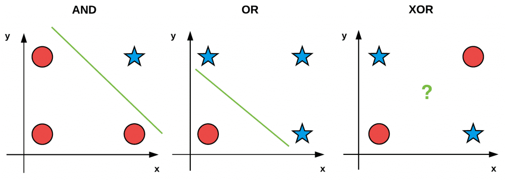
We often use these simple “bitwise datasets” to test and debug machine learning algorithms. If we plot and visualize the AND, OR, and XOR values (with red circles being zero outputs and blue stars one outputs) in Figure 1, you’ll notice an interesting pattern:

Figure 1: Both the AND and OR bitwise datasets are linearly separable, meaning that we can draw a single line (green) that separates the two classes. However, for XOR it is impossible to draw a single line that separates the two classes — this is therefore a nonlinearly separable dataset.

Both AND and OR are linearly separable — we can clearly draw a line that separates the 0 and 1 classes — the same is not true for XOR. Take the time now to convince yourself that it is not possible to draw a line that cleanly separates the two classes in the XOR problem. XOR is, therefore, an example of a nonlinearly separable dataset.

Ideally, we would like our machine learning algorithms to be able to separate nonlinear classes as most datasets encountered in the real world are nonlinear. Therefore, when constructing, debugging, and evaluating a given machine learning algorithm, we may use the bitwise values x0 and x1 as our design matrix and then try to predict the corresponding y values.

Unlike our standard procedure of splitting our data into training and testing splits, when using bitwise datasets we simply train and evaluate our network on the same set of data. Our goal here is simply to determine if it’s even possible for our learning algorithm to learn the patterns in the data. As we’ll find out, the Perceptron algorithm can correctly classify the AND and OR functions but fails to classify the XOR data.

Perceptron Architecture

Rosenblatt (1958) defined a Perceptron as a system that learns using labeled examples (i.e., supervised learning) of feature vectors (or raw pixel intensities), mapping these inputs to their corresponding output class labels.

In its simplest form, a Perceptron contains N input nodes, one for each entry in the input row of the design matrix, followed by only one layer in the network with just a single node in that layer (Figure 2).

There exist connections and their corresponding weights w1, w2, …, wi from the input xi’s to the single output node in the network. This node takes the weighted sum of inputs and applies a step function to determine the output class label. The Perceptron outputs either a 0 or a 1 — 0 for class #1 and 1 for class #2; thus, in its original form, the Perceptron is simply a binary, two-class classifier.

Figure 2: Architecture of the Perceptron network. 1. Initialize our weight vector w with small random values
2. Until Perceptron converges:
(a) Loop over each feature vector xj and true class label di in our training set D
(b) Take x and pass it through the network, calculating the output value: yj = f(w(t) · xj)
(c) Update the weights w: wi(t +1) = wi(t) +α(dj −yj)xj,i for all features 0 <= i <= nFigure 3: The Perceptron algorithm training procedure.

Perceptron Training Procedure and the Delta Rule

Training a Perceptron is a fairly straightforward operation. Our goal is to obtain a set of weights w that accurately classifies each instance in our training set. In order to train our Perceptron, we iteratively feed the network with our training data multiple times. Each time the network has seen the full set of training data, we say an epoch has passed. It normally takes many epochs until a weight vector w can be learned to linearly separate our two classes of data.

The pseudocode for the Perceptron training algorithm can be found below:

The actual “learning” takes place in Steps 2b and 2c. First, we pass the feature vector xj through the network, take the dot product with the weights w and obtain the output yj. This value is then passed through the step function which will return 1 if x > 0 and 0 otherwise.

Now we need to update our weight vector w to step in the direction that is “closer” to the correct classification. This update of the weight vector is handled by the delta rule in Step 2c.

The expression (dj −yj) determines if the output classification is correct or not. If the classification is correct, then this difference will be zero. Otherwise, the difference will be either positive or negative, giving us the direction in which our weights will be updated (ultimately bringing us closer to the correct classification). We then multiply (dj − yj) by xj, moving us closer to the correct classification.

The value α is our learning rate and controls how large (or small) of a step we take. It’s critical that this value is set correctly. A larger value of α will cause us to take a step in the right direction; however, this step could be too large, and we could easily overstep a local/global optimum.

Conversely, a small value of α allows us to take tiny baby steps in the right direction, ensuring we don’t overstep a local/global minimum; however, these tiny baby steps may take an intractable amount of time for our learning to converge.

Finally, we add in the previous weight vector at time t, wj(t) which completes the process of “stepping” towards the correct classification. If you find this training procedure a bit confusing, don’t worry.

Perceptron Training Termination

The Perceptron training process is allowed to proceed until all training samples are classified correctly or a preset number of epochs is reached. Termination is ensured if α is sufficiently small and the training data is linearly separable.

So, what happens if our data is not linearly separable or we make a poor choice in α? Will training continue infinitely? In this case, no — we normally stop after a set number of epochs has been hit or if the number of misclassifications has not changed in a large number of epochs (indicating that the data is not linearly separable). For more details on the perceptron algorithm, please refer to either Andrew Ng’s Stanford lecture or the introductory chapters of Mehrota et al. (1997).

Implementing the Perceptron in Python

Now that we have studied the Perceptron algorithm, let’s implement the actual algorithm in Python. Create a file named perceptron.py in your pyimagesearch.nn package — this file will store our actual Perceptron implementation:

|--- pyimagesearch
|    |--- __init__.py
|    |--- nn
|    |    |--- __init__.py
|    |    |--- perceptron.py

After you’ve created the file, open it, and insert the following code:

# import the necessary packages
import numpy as np

class Perceptron:
	def __init__(self, N, alpha=0.1):
		# initialize the weight matrix and store the learning rate
		self.W = np.random.randn(N + 1) / np.sqrt(N)
		self.alpha = alpha

Line 5 defines the constructor to our Perceptron class, which accepts a single required parameter followed by a second optional one:

N: The number of columns in our input feature vectors. In the context of our bitwise datasets, we’ll set N equal to two since there are two inputs.
alpha: Our learning rate for the Perceptron algorithm. We’ll set this value to 0.1 by default. Common choices of learning rates are normally in the range α = 0.1, 0.01, 0.001.

Line 7 files our weight matrix W with random values sampled from a “normal” (Gaussian) distribution with zero mean and unit variance. The weight matrix will have N +1 entries, one for each of the N inputs in the feature vector, plus one for the bias. We divide W by the square-root of the number of inputs, a common technique used to scale our weight matrix, leading to faster convergence. We will cover weight initialization techniques later in this chapter.

Next, let’s define the step function:

	def step(self, x):
		# apply the step function
		return 1 if x > 0 else 0

This function mimics the behavior of the step equation — if x is positive we return 1, otherwise, we return 0.

To actually train the Perceptron we’ll define a function named fit. If you have any previous experience with machine learning, Python, and the scikit-learn library then you’ll know that it’s common to name your training procedure function fit, as in “fit a model to the data”:

	def fit(self, X, y, epochs=10):
		# insert a column of 1's as the last entry in the feature
		# matrix -- this little trick allows us to treat the bias
		# as a trainable parameter within the weight matrix
		X = np.c_[X, np.ones((X.shape[0]))]

The fit method requires two parameters followed by a single optional one:

The X value is our actual training data. The y variable is our target output class labels (i.e., what our network should be predicting). Finally, we supply epochs, the number of epochs our Perceptron will train for.

Line 18 applies the bias trick by inserting a column of ones into the training data, which allows us to treat the bias as a trainable parameter directly inside the weight matrix.

Next, let’s review the actual training procedure:

		# loop over the desired number of epochs
		for epoch in np.arange(0, epochs):
			# loop over each individual data point
			for (x, target) in zip(X, y):
				# take the dot product between the input features
				# and the weight matrix, then pass this value
				# through the step function to obtain the prediction
				p = self.step(np.dot(x, self.W))

				# only perform a weight update if our prediction
				# does not match the target
				if p != target:
					# determine the error
					error = p - target

					# update the weight matrix
					self.W += -self.alpha * error * x

On Line 21, we start looping over the desired number of epochs. For each epoch, we also loop over each individual data point x and output target class label (Line 23).

Line 27 takes the dot product between the input features x and the weight matrix W, then passes the output through the step function to obtain the prediction by the Perceptron.

Applying the same training procedure detailed in Figure 3, we only perform a weight update if our prediction does not match the target (Line 31). If this is the case, we determine the error (Line 33) by computing the sign (either positive or negative) via the difference operation.

Updating the weight matrix is handled on Line 36 where we take a step towards the correct classification, scaling this step by our learning rate alpha. Over a series of epochs, our Perceptron is able to learn patterns in the underlying data and shift the values of the weight matrix such that we correctly classify our input samples x.

The last function we need to define is predict, which, as the name suggests, is used to predict the class labels for a given set of input data:

	def predict(self, X, addBias=True):
		# ensure our input is a matrix
		X = np.atleast_2d(X)

		# check to see if the bias column should be added
		if addBias:
			# insert a column of 1's as the last entry in the feature
			# matrix (bias)
			X = np.c_[X, np.ones((X.shape[0]))]

		# take the dot product between the input features and the
		# weight matrix, then pass the value through the step
		# function
		return self.step(np.dot(X, self.W))

Our predict method requires a set of input data X that needs to be classified. A check on Line 43 is made to see if a bias column needs to be added.

Obtaining the output predictions for X is the same as the training procedure — simply take the dot product between the input features X and our weight matrix W, and then pass the value through our step function. The output of the step function is returned to the calling function.

Now that we’ve implemented our Perceptron class, let’s try to apply it to our bitwise datasets and see how the neural network performs.

Evaluating the Perceptron Bitwise Datasets

To start, let’s create a file named perceptron_or.py that attempts to fit a Perceptron model to the bitwise OR dataset:

# import the necessary packages
from pyimagesearch.nn import Perceptron
import numpy as np

# construct the OR dataset
X = np.array([[0, 0], [0, 1], [1, 0], [1, 1]])
y = np.array([[0], [1], [1], [1]])

# define our perceptron and train it
print("[INFO] training perceptron...")
p = Perceptron(X.shape[1], alpha=0.1)
p.fit(X, y, epochs=20)

Lines 2 and 3 import our required Python packages. We’ll be using our Perceptron implementation. Lines 6 and 7 define the OR dataset based on Table 1.

Lines 11 and 12 train our Perceptron with a learning rate of α = 0.1 for a total of 20 epochs.

We can then evaluate our Perceptron on the data to validate that it did, in fact, learn the OR function:

# now that our perceptron is trained we can evaluate it
print("[INFO] testing perceptron...")

# now that our network is trained, loop over the data points
for (x, target) in zip(X, y):
	# make a prediction on the data point and display the result
	# to our console
	pred = p.predict(x)
	print("[INFO] data={}, ground-truth={}, pred={}".format(
		x, target[0], pred))

On Line 18, we loop over each of the data points in the OR dataset. For each of these data points, we pass it through the network and obtain the prediction (Line 21).

Finally, Lines 22 and 23 display the input data point, the ground-truth label, as well as our predicted label to our console.

To see if our Perceptron algorithm is able to learn the OR function, just execute the following command:

$ python perceptron_or.py 
[INFO] training perceptron...
[INFO] testing perceptron...
[INFO] data=[0 0], ground-truth=0, pred=0
[INFO] data=[0 1], ground-truth=1, pred=1
[INFO] data=[1 0], ground-truth=1, pred=1
[INFO] data=[1 1], ground-truth=1, pred=1

Sure enough, our neural network is able to correctly predict that the OR operation for x0 = 0 and x1 = 0 is zero — all other combinations are one.

Now, let’s move on to the AND function — create a new file named perceptron_and.py and insert the following code:

# import the necessary packages
from pyimagesearch.nn import Perceptron
import numpy as np

# construct the AND dataset
X = np.array([[0, 0], [0, 1], [1, 0], [1, 1]])
y = np.array([[0], [0], [0], [1]])

# define our perceptron and train it
print("[INFO] training perceptron...")
p = Perceptron(X.shape[1], alpha=0.1)
p.fit(X, y, epochs=20)

# now that our perceptron is trained we can evaluate it
print("[INFO] testing perceptron...")

# now that our network is trained, loop over the data points
for (x, target) in zip(X, y):
	# make a prediction on the data point and display the result
	# to our console
	pred = p.predict(x)
	print("[INFO] data={}, ground-truth={}, pred={}".format(
		x, target[0], pred))

Notice here that the only lines of code that have changed are Lines 6 and 7 where we define the AND dataset rather than the OR dataset.

Executing the following command, we can evaluate the Perceptron on the AND function:

$ python perceptron_and.py 
[INFO] training perceptron...
[INFO] testing perceptron...
[INFO] data=[0 0], ground-truth=0, pred=0
[INFO] data=[0 1], ground-truth=0, pred=0
[INFO] data=[1 0], ground-truth=0, pred=0
[INFO] data=[1 1], ground-truth=1, pred=1

Again, our Perceptron was able to correctly model the function. The AND function is only true when both x0 = 1 and x1 = 1 – for all other combinations the bitwise AND is zero.

Finally, let’s take a look at the nonlinearly separable XOR function inside perceptron_xor.py:

# import the necessary packages
from pyimagesearch.nn import Perceptron
import numpy as np

# construct the XOR dataset
X = np.array([[0, 0], [0, 1], [1, 0], [1, 1]])
y = np.array([[0], [1], [1], [0]])

# define our perceptron and train it
print("[INFO] training perceptron...")
p = Perceptron(X.shape[1], alpha=0.1)
p.fit(X, y, epochs=20)

# now that our perceptron is trained we can evaluate it
print("[INFO] testing perceptron...")

# now that our network is trained, loop over the data points
for (x, target) in zip(X, y):
	# make a prediction on the data point and display the result
	# to our console
	pred = p.predict(x)
	print("[INFO] data={}, ground-truth={}, pred={}".format(
		x, target[0], pred))

Again, the only lines of code that have been changed are Lines 6 and 7 where we define the XOR data. The XOR operator is true if and only if one (but not both) x’s are one.

Executing the following command we can see that the Perceptron cannot learn this nonlinear relationship:

$ python perceptron_xor.py 
[INFO] training perceptron...
[INFO] testing perceptron...
[INFO] data=[0 0], ground-truth=0, pred=1
[INFO] data=[0 1], ground-truth=1, pred=1
[INFO] data=[1 0], ground-truth=1, pred=0
[INFO] data=[1 1], ground-truth=0, pred=0

No matter how many times you run this experiment with varying learning rates or different weight initialization schemes, you will never be able to correctly model the XOR function with a single layer Perceptron. Instead, what we need is more layers with nonlinear activation functions and with that, comes the start of deep learning.

Download the Source Code and FREE 17-page Resource Guide

Enter your email address below to get a .zip of the code and a FREE 17-page Resource Guide on Computer Vision, OpenCV, and Deep Learning. Inside you’ll find my hand-picked tutorials, books, courses, and libraries to help you master CV and DL!