
Implementing feedforward neural networks with Keras and TensorFlow – PyImageSearch
Now that we have implemented neural networks in pure Python, let’s move on to the preferred implementation method — using a dedicated (highly optimized) neural network library such as Keras.

Today, I will discuss how to implement feedforward, multi-layer networks and apply them to the MNIST and CIFAR-10 datasets. These result will hardly be “state-of-the-art,” but will serve two purposes:
- To demonstrate how you can implement simple neural networks using the Keras library.
- Obtain a baseline using standard neural networks which we will later compare to Convolutional Neural Networks (noting that CNNS will dramatically outperform our previous methods).
![]()
Mục Lục
Looking for the source code to this post?
Jump Right To The Downloads Section
MNIST
Today, we’ll be using the full MNIST dataset, consisting of 70,000 data points (7,000 examples per digit). Each data point is represented by a 784-d vector, corresponding to the (flattened) 28×28 images in the MNIST dataset. Our goal is to train a neural network (using Keras) to obtain > 90% accuracy on this dataset.
As we’ll find out, using Keras to build our network architecture is substantially easier than our pure Python version. In fact, the actual network architecture will only occupy four lines of code — the rest of the code in this example simply involves loading the data from disk, transforming the class labels, and then displaying the results.
To get started, open a new file, name it keras_mnist.py, and insert the following code:
# import the necessary packages
from sklearn.preprocessing import LabelBinarizer
from sklearn.metrics import classification_report
from tensorflow.keras.models import Sequential
from tensorflow.keras.layers import Dense
from tensorflow.keras.optimizers import SGD
from tensorflow.keras.datasets import mnist
from tensorflow.keras import backend as K
import matplotlib.pyplot as plt
import numpy as np
import argparse
Lines 2-11 import our required Python packages. The LabelBinarizer will be used to one-hot encode our integer labels as vector labels. One-hot encoding transforms categorical labels from a single integer to a vector. Many machine learning algorithms (including neural networks) benefit from this type of label representation. I’ll be discussing one-hot encoding in more detail and providing multiple examples (including using the LabelBinarizer) later in this section.
The classification_report function will give us a nicely formatted report displaying the total accuracy of our model, along with a breakdown on the classification accuracy for each digit.
Lines 4-6 import the necessary packages to create a simple feedforward neural network with Keras. The Sequential class indicates that our network will be feedforward and layers will be added to the class sequentially, one on top of the other. The Dense class on Line 5 is the implementation of our fully connected layers. For our network to actually learn, we need to apply SGD (Line 6) to optimize the parameters of the network. Finally, to gain access to full MNIST dataset, we need to import the mnist helper function on Line 7.
Let’s move on to parsing our command line arguments:
# construct the argument parse and parse the arguments
ap = argparse.ArgumentParser()
ap.add_argument("-o", "--output", required=True,
	help="path to the output loss/accuracy plot")
args = vars(ap.parse_args())
We only need a single switch here, --output, which is the path to where our figure plotting the loss and accuracy over time will be saved to disk.
Next, let’s load the full MNIST dataset:
# grab the MNIST dataset (if this is your first time using this
# dataset then the 11MB download may take a minute)
print("[INFO] accessing MNIST...")
((trainX, trainY), (testX, testY)) = mnist.load_data()

# each image in the MNIST dataset is represented as a 28x28x1
# image, but in order to apply a standard neural network we must
# first "flatten" the image to be simple list of 28x28=784 pixels
trainX = trainX.reshape((trainX.shape[0], 28 * 28 * 1))
testX = testX.reshape((testX.shape[0], 28 * 28 * 1))

# scale data to the range of [0, 1]
trainX = trainX.astype("float32") / 255.0
testX = testX.astype("float32") / 255.0
Line 22 loads the MNIST dataset from disk. If you have never run this function before, then the MNIST dataset will be downloaded and stored locally to your machine. Once the dataset has been downloaded, it is cached to your machine and will not have to be downloaded again.
Each image in the MNIST dataset is represented as 28×28×1 pixel image. In order to train our neural network on the image data we first need to flatten the 2D images into a flat list of 28×28 = 784 values (Lines 27 and 28).
We then perform data normalization on Lines 31 and 32 by scaling the pixel intensities to the range [0, 1].
Given the training and testing splits, we can now encode our labels:
# convert the labels from integers to vectors
lb = LabelBinarizer()
trainY = lb.fit_transform(trainY)
testY = lb.transform(testY)
Each data point in the MNIST dataset has an integer label in the range [0, 9], one for each of the possible ten digits in the MNIST dataset. A label with a value of 0 indicates that the corresponding image contains a zero digit. Similarly, a label with a value of 8 indicates that the corresponding image contains the number eight.
However, we first need to transform these integer labels into vector labels, where the index in the vector for label is set to 1 and 0 otherwise (this process is called one-hot encoding).
For example, consider the label 3 and we wish to binarize/one-hot encode it — the label 3 now becomes:
[0, 0, 0, 1, 0, 0, 0, 0, 0, 0]
Notice how only the index for the digit three is set to one — all other entries in the vector are set to zero. Astute readers may wonder why the fourth and not the third entry in the vector is updated? Recall that the first entry in the label is actually for the digit zero. Therefore, the entry for the digit three is actually the fourth index in the list.
Here is a second example, this time with the label 1 binarized:
[0, 1, 0, 0, 0, 0, 0, 0, 0, 0]
The second entry in the vector is set to one (since the first entry corresponds to the label 0), while all other entries are set to zero.
I have included the one-hot encoding representations for each digit, 0−9, in the listing below:
0: [1, 0, 0, 0, 0, 0, 0, 0, 0, 0]
1: [0, 1, 0, 0, 0, 0, 0, 0, 0, 0]
2: [0, 0, 1, 0, 0, 0, 0, 0, 0, 0]
3: [0, 0, 0, 1, 0, 0, 0, 0, 0, 0]
4: [0, 0, 0, 0, 1, 0, 0, 0, 0, 0]
5: [0, 0, 0, 0, 0, 1, 0, 0, 0, 0]
6: [0, 0, 0, 0, 0, 0, 1, 0, 0, 0]
7: [0, 0, 0, 0, 0, 0, 0, 1, 0, 0]
8: [0, 0, 0, 0, 0, 0, 0, 0, 1, 0]
9: [0, 0, 0, 0, 0, 0, 0, 0, 0, 1]
This encoding may seem tedious, but many machine learning algorithms (including neural networks), benefit from this label representation. Luckily, most machine learning software packages provide a method/function to perform one-hot encoding, removing much of the tediousness.
Lines 35-37 simply perform this process of one-hot encoding the input integer labels as vector labels for both the training and testing set.
Next, let’s define our network architecture:
# define the 784-256-128-10 architecture using Keras
model = Sequential()
model.add(Dense(256, input_shape=(784,), activation="sigmoid"))
model.add(Dense(128, activation="sigmoid"))
model.add(Dense(10, activation="softmax"))
As you can see, our network is a feedforward architecture, instantiated by the Sequential class on Line 40 — this architecture implies that the layers will be stacked on top of each other with the output of the previous layer feeding into the next.
Line 41 defines the first fully connected layer in the network. The input_shape is set to 784, the dimensionality of each MNIST data points. We then learn 256 weights in this layer and apply the sigmoid activation function. The next layer (Line 42) learns 128 weights. Finally, Line 43 applies another fully connected layer, this time only learning 10 weights, corresponding to the ten (0-9) output classes. Instead of a sigmoid activation, we’ll use a softmax activation to obtain normalized class probabilities for each prediction.
Let’s go ahead and train our network:
# train the model using SGD
print("[INFO] training network...")
sgd = SGD(0.01)
model.compile(loss="categorical_crossentropy", optimizer=sgd,
	metrics=["accuracy"])
H = model.fit(trainX, trainY, validation_data=(testX, testY),
	epochs=100, batch_size=128)
On Line 47, we initialize the SGD optimizer with a learning rate of 0.01 (which we may commonly write as 1e-2). We’ll use the category cross-entropy loss function as our loss metric (Lines 48 and 49). Using the cross-entropy loss function is also why we had to convert our integer labels to vector labels.
A call to .fit of the model on Lines 50 and 51 kicks off the training of our neural network. We’ll supply the training data and training labels as the first two arguments to the method.
The validation_data can then be supplied, which is our testing split. In most circumstances, such as when you are tuning hyperparameters or deciding on a model architecture, you’ll want your validation set to be a true validation set and not your testing data. In this case, we are simply demonstrating how to train a neural network from scratch using Keras so we’re being a bit lenient with our guidelines.
We’ll allow our network to train for a total of 100 epochs using a batch size of 128 data points at a time. The method returns a dictionary, H, which we’ll use to plot the loss/accuracy of the network over time in a couple of code blocks.
Once the network has finished training, we’ll want to evaluate it on the testing data to obtain our final classifications:
# evaluate the network
print("[INFO] evaluating network...")
predictions = model.predict(testX, batch_size=128)
print(classification_report(testY.argmax(axis=1),
	predictions.argmax(axis=1),
	target_names=[str(x) for x in lb.classes_]))
A call to the .predict method of model will return the class label probabilities for every data point in testX (Line 55). Thus, if you were to inspect the predictions NumPy array it would have the shape (X, 10) as there are 17,500 total data points in the testing set and ten possible class labels (the digits 0-9).
Each entry in a given row is, therefore, a probability. To determine the class with the largest probability, we can simply call .argmax(axis=1) as we do on Line 56, which will give us the index of the class label with the largest probability, and, therefore, our final output classification. The final output classification by the network is tabulated, and then a final classification report is displayed to our console on Lines 56-58.
Our final code block handles plotting the training loss, training accuracy, validation loss, and validation accuracy over time:
# plot the training loss and accuracy
plt.style.use("ggplot")
plt.figure()
plt.plot(np.arange(0, 100), H.history["loss"], label="train_loss")
plt.plot(np.arange(0, 100), H.history["val_loss"], label="val_loss")
plt.plot(np.arange(0, 100), H.history["accuracy"], label="train_acc")
plt.plot(np.arange(0, 100), H.history["val_accuracy"], label="val_acc")
plt.title("Training Loss and Accuracy")
plt.xlabel("Epoch #")
plt.ylabel("Loss/Accuracy")
plt.legend()
plt.savefig(args["output"])
This plot is then saved to disk based on the --output command line argument. To train our network of fully connected layers on MNIST, just execute the following command:
$ python keras_mnist.py --output output/keras_mnist.png
[INFO] loading MNIST (full) dataset...
[INFO] training network...
Train on 52500 samples, validate on 17500 samples
Epoch 1/100
1s - loss: 2.2997 - acc: 0.1088 - val_loss: 2.2918 - val_acc: 0.1145
Epoch 2/100
1s - loss: 2.2866 - acc: 0.1133 - val_loss: 2.2796 - val_acc: 0.1233
Epoch 3/100
1s - loss: 2.2721 - acc: 0.1437 - val_loss: 2.2620 - val_acc: 0.1962
...
Epoch 98/100
1s - loss: 0.2811 - acc: 0.9199 - val_loss: 0.2857 - val_acc: 0.9153
Epoch 99/100
1s - loss: 0.2802 - acc: 0.9201 - val_loss: 0.2862 - val_acc: 0.9148
Epoch 100/100
1s - loss: 0.2792 - acc: 0.9204 - val_loss: 0.2844 - val_acc: 0.9160
[INFO] evaluating network...
             precision    recall  f1-score   support

        0.0       0.94      0.96      0.95      1726
        1.0       0.95      0.97      0.96      2004
        2.0       0.91      0.89      0.90      1747
        3.0       0.91      0.88      0.89      1828
        4.0       0.91      0.93      0.92      1686
        5.0       0.89      0.86      0.88      1581
        6.0       0.92      0.96      0.94      1700
        7.0       0.92      0.94      0.93      1814
        8.0       0.88      0.88      0.88      1679
        9.0       0.90      0.88      0.89      1735

avg / total       0.92      0.92      0.92     17500
As the results demonstrate, we are obtaining ≈92% accuracy. Furthermore, the training and validation curves match each other nearly identically (Figure 1), indicating there is no overfitting or issues with the training process.
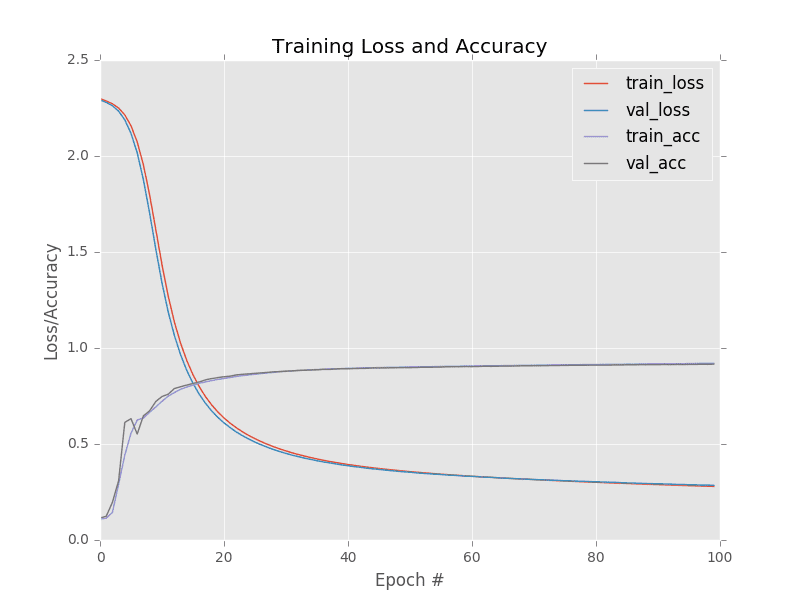 Figure 1: Training a 784−256−128−10 feedforward neural network with Keras on the full MNIST dataset. Notice how our training and validation curves are near identical, implying there is no overfitting occurring.
In fact, if you are unfamiliar with the MNIST dataset, you might think 92% accuracy is excellent — and it was, perhaps 20 years ago. Using Convolutional Neural Networks, we can easily obtain > 98% accuracy. Current state-of-the-art approaches can even break 99% accuracy.
While on the surface it may appear that our (strictly) fully connected network is performing well, we can actually do much better. And as we’ll see in the next section, strictly fully connected networks applied to more challenging datasets can in some cases do just barely better than guessing randomly.
CIFAR-10
When it comes to computer vision and machine learning, the MNIST dataset is the classic definition of a “benchmark” dataset, one that is too easy to obtain high accuracy results on, and not representative of the images we’ll see in the real world.
For a more challenging benchmark dataset, we commonly use CIFAR-10, a collection of 60,000, 32×32 RGB images, thus implying that each image in the dataset is represented by 32×32×3 = 3,072 integers. As the name suggests, CIFAR-10 consists of 10 classes, including airplane, automobile, bird, cat, deer, dog, frog, horse, ship, and truck. A sample of the CIFAR-10 dataset for each class can be seen in Figure 2.
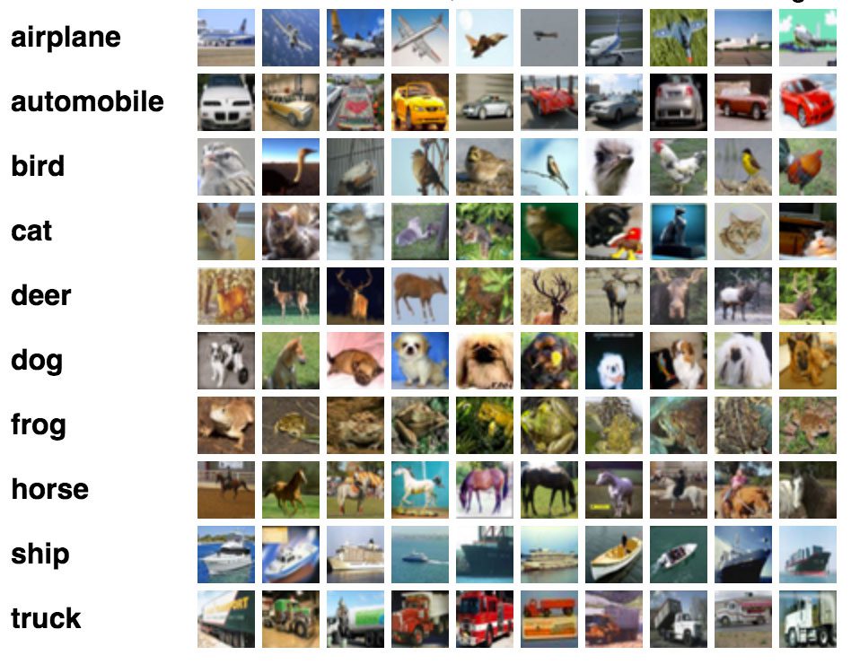 Figure 2: Example images from the ten class CIFAR-10 dataset.
Each class is evenly represented with 6,000 images per class. When training and evaluating a machine learning model on CIFAR-10, it’s typical to use the predefined data splits by the authors and use 50,000 images for training and 10,000 for testing.
CIFAR-10 is substantially harder than the MNIST dataset. The challenge comes from the dramatic variance in how objects appear. For example, we can no longer assume that an image containing a green pixel at a given (x, y)-coordinate is a frog. This pixel could be a background of a forest that contains a deer. Or it could be the color of a green car or truck.
These assumptions are a stark contrast to the MNIST dataset, where the network can learn assumptions regarding the spatial distribution of pixel intensities. For example, the spatial distribution of foreground pixels of a 1 is substantially different than a 0 or a 5. This type of variance in object appearance makes applying a series of fully connected layers much more challenging. As we’ll find out in the rest of this section, standard FC (fully connected) layer networks are not suited for this type of image classification.
Let’s go ahead and get started. Open a new file, name it keras_cifar10.py, and insert the following code:
# import the necessary packages
from sklearn.preprocessing import LabelBinarizer
from sklearn.metrics import classification_report
from tensorflow.keras.models import Sequential
from tensorflow.keras.layers import Dense
from tensorflow.keras.optimizers import SGD
from tensorflow.keras.datasets import cifar10
import matplotlib.pyplot as plt
import numpy as np
import argparse
Lines 2-10 import our required Python packages to build our fully connected network, identical to the previous section with MNIST. The exception is the special utility function on Line 7 — since CIFAR-10 is such a common dataset that researchers benchmark machine learning and deep learning algorithms on, it’s common to see deep learning libraries provide simple helper functions to automatically load this dataset from disk.
Next, we can parse our command line arguments:
# construct the argument parse and parse the arguments
ap = argparse.ArgumentParser()
ap.add_argument("-o", "--output", required=True,
	help="path to the output loss/accuracy plot")
args = vars(ap.parse_args())
The only command line argument we need is --output, the path to our output loss/accuracy plot.
Let’s go ahead and load the CIFAR-10 dataset:
# load the training and testing data, scale it into the range [0, 1],
# then reshape the design matrix
print("[INFO] loading CIFAR-10 data...")
((trainX, trainY), (testX, testY)) = cifar10.load_data()
trainX = trainX.astype("float") / 255.0
testX = testX.astype("float") / 255.0
trainX = trainX.reshape((trainX.shape[0], 3072))
testX = testX.reshape((testX.shape[0], 3072))
A call to cifar10.load_data on Line 21 automatically loads the CIFAR-10 dataset from disk, pre-segmented into training and testing split. If this is the first time you are calling cifar10.load_data, then this function will fetch and download the dataset for you. This file is ≈170MB, so be patient as it is downloaded and unarchived. Once the file is downloaded once, it will be cached locally on your machine and will not have to be downloaded again.
Lines 22 and 23 convert the data type of CIFAR-10 from unsigned 8-bit integers to floating point, followed by scaling the data to the range [0, 1]. Lines 24 and 25 are responsible for reshaping the design matrix for the training and testing data. Recall that each image in the CIFAR-10 dataset is represented by a 32×32×3 image.
For example, trainX has the shape (50000, 32, 32, 3) and testX has the shape (10000, 32, 32, 3). If we were to flatten this image into a single list of floating point values, the list would have a total of 32×32×3 = 3,072 total entries in it.
To flatten each of the images in the training and testing sets, we simply use the .reshape function of NumPy. After this function executes, trainX now has the shape (50000, 3072) while testX has the shape (10000, 3072).
Now that the CIFAR-10 dataset has been loaded from disk, let’s once again binarize the class label integers into vectors, followed by initializing a list of the actual names of the class labels:
# convert the labels from integers to vectors
lb = LabelBinarizer()
trainY = lb.fit_transform(trainY)
testY = lb.transform(testY)

# initialize the label names for the CIFAR-10 dataset
labelNames = ["airplane", "automobile", "bird", "cat", "deer",
	"dog", "frog", "horse", "ship", "truck"]
It’s now time to define the network architecture:
# define the 3072-1024-512-10 architecture using Keras
model = Sequential()
model.add(Dense(1024, input_shape=(3072,), activation="relu"))
model.add(Dense(512, activation="relu"))
model.add(Dense(10, activation="softmax"))
Line 37 instantiates the Sequential class. We then add the first Dense layer which has an input_shape of 3072, a node for each of the 3,072 flattened pixel values in the design matrix — this layer is then responsible for learning 1,024 weights. We’ll also swap out the antiquated sigmoid for a ReLU activation in hopes of improving network performance.
The next fully connected layer (Line 39) learns 512 weights, while the final layer (Line 40) learns weights corresponding to ten possible output classifications, along with a softmax classifier to obtain the final output probabilities for each class.
Now that the architecture of the network is defined, we can train it:
# train the model using SGD
print("[INFO] training network...")
sgd = SGD(0.01)
model.compile(loss="categorical_crossentropy", optimizer=sgd,
	metrics=["accuracy"])
H = model.fit(trainX, trainY, validation_data=(testX, testY),
	epochs=100, batch_size=32)
We’ll use the SGD optimizer to train the network with a learning rate of 0.01, a fairly standard initial choice. The network will be trained for a total of 100 epochs using batches of 32.
Once the network has been trained, we can evaluate it using classification_report to obtain a more detailed review of model performance:
# evaluate the network
print("[INFO] evaluating network...")
predictions = model.predict(testX, batch_size=32)
print(classification_report(testY.argmax(axis=1),
	predictions.argmax(axis=1), target_names=labelNames))
And finally, we’ll also plot the loss/accuracy over time as well:
# plot the training loss and accuracy
plt.style.use("ggplot")
plt.figure()
plt.plot(np.arange(0, 100), H.history["loss"], label="train_loss")
plt.plot(np.arange(0, 100), H.history["val_loss"], label="val_loss")
plt.plot(np.arange(0, 100), H.history["accuracy"], label="train_acc")
plt.plot(np.arange(0, 100), H.history["val_accuracy"], label="val_acc")
plt.title("Training Loss and Accuracy")
plt.xlabel("Epoch #")
plt.ylabel("Loss/Accuracy")
plt.legend()
plt.savefig(args["output"])
To train our network on CIFAR-10, open up a terminal and execute the following command:
$ python keras_cifar10.py --output output/keras_cifar10.png
[INFO] training network...
Train on 50000 samples, validate on 10000 samples
Epoch 1/100
7s - loss: 1.8409 - acc: 0.3428 - val_loss: 1.6965 - val_acc: 0.4070
Epoch 2/100
7s - loss: 1.6537 - acc: 0.4160 - val_loss: 1.6561 - val_acc: 0.4163
Epoch 3/100
7s - loss: 1.5701 - acc: 0.4449 - val_loss: 1.6049 - val_acc: 0.4376
...
Epoch 98/100
7s - loss: 0.0292 - acc: 0.9969 - val_loss: 2.2477 - val_acc: 0.5712
Epoch 99/100
7s - loss: 0.0272 - acc: 0.9972 - val_loss: 2.2514 - val_acc: 0.5717
Epoch 100/100
7s - loss: 0.0252 - acc: 0.9976 - val_loss: 2.2492 - val_acc: 0.5739
[INFO] evaluating network...
             precision    recall  f1-score   support

   airplane       0.63      0.66      0.64      1000
 automobile       0.69      0.65      0.67      1000
       bird       0.48      0.43      0.45      1000
        cat       0.40      0.38      0.39      1000
       deer       0.52      0.51      0.51      1000
        dog       0.48      0.47      0.48      1000
       frog       0.64      0.63      0.64      1000
      horse       0.63      0.62      0.63      1000
       ship       0.64      0.74      0.69      1000
      truck       0.59      0.65      0.62      1000

avg / total       0.57      0.57      0.57     10000
Looking at the output, you can see that our network obtained 57% accuracy. Examining our plot of loss and accuracy over time (Figure 3), we can see that our network struggles with overfitting past epoch 10. Loss initially starts to decrease, levels out a bit, and then skyrockets, and never comes down again. All the while training loss is falling consistently epoch-over-epoch. This behavior of decreasing training loss while validation loss increases is indicative of extreme overfitting.
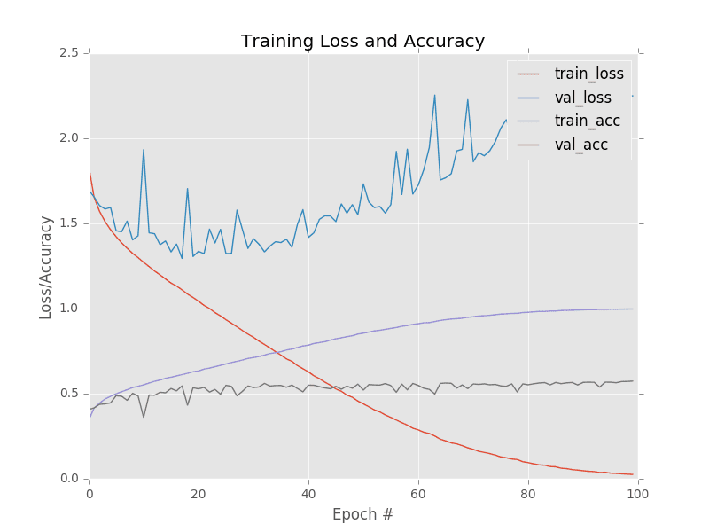 Figure 3: Using a standard feedforward neural network leads to dramatic overfitting in the more challenging CIFAR-10 dataset (notice how training loss falls while validation loss rises dramatically). To be successful at the CIFAR-10 challenge, we’ll need a powerful technique — Convolutional Neural Networks.
We could certainly consider optimizing our hyperparameters further, in particular, experimenting with varying learning rates and increasing both the depth and the number of nodes in the network, but we would be fighting for meager gains.
The fact is this — basic feedforward networks with strictly fully connected layers are not suitable for challenging image datasets. For that, we need a more advanced approach: Convolutional Neural Networks.
What’s next? I recommend PyImageSearch University.
Course information:
69 total classes • 73 hours of on-demand code walkthrough videos • Last updated: February 2023
★★★★★
4.84 (128 Ratings) • 15,800+ Students Enrolled
I strongly believe that if you had the right teacher you could master computer vision and deep learning.
Do you think learning computer vision and deep learning has to be time-consuming, overwhelming, and complicated? Or has to involve complex mathematics and equations? Or requires a degree in computer science?
That’s not the case.
All you need to master computer vision and deep learning is for someone to explain things to you in simple, intuitive terms. And that’s exactly what I do. My mission is to change education and how complex Artificial Intelligence topics are taught.
If you’re serious about learning computer vision, your next stop should be PyImageSearch University, the most comprehensive computer vision, deep learning, and OpenCV course online today. Here you’ll learn how to successfully and confidently apply computer vision to your work, research, and projects. Join me in computer vision mastery.
Inside PyImageSearch University you’ll find:
- ✓ 69 courses on essential computer vision, deep learning, and OpenCV topics
- ✓ 69 Certificates of Completion
- ✓ 73 hours of on-demand video
- ✓ Brand new courses released regularly, ensuring you can keep up with state-of-the-art techniques
- ✓ Pre-configured Jupyter Notebooks in Google Colab
- ✓ Run all code examples in your web browser — works on Windows, macOS, and Linux (no dev environment configuration required!)
- ✓ Access to centralized code repos for all 500+ tutorials on PyImageSearch
- ✓ Easy one-click downloads for code, datasets, pre-trained models, etc.
- ✓ Access on mobile, laptop, desktop, etc.
Click here to join PyImageSearch University

Download the Source Code and FREE 17-page Resource Guide
Enter your email address below to get a .zip of the code and a FREE 17-page Resource Guide on Computer Vision, OpenCV, and Deep Learning. Inside you’ll find my hand-picked tutorials, books, courses, and libraries to help you master CV and DL!


![Toni Kroos là ai? [ sự thật về tiểu sử đầy đủ Toni Kroos ]](https://evbn.org/wp-content/uploads/New-Project-6635-1671934592.jpg)


