Hyperparameter tuning for Deep Learning with scikit-learn, Keras, and TensorFlow

In this tutorial, you will learn how to tune the hyperparameters of a deep neural network using scikit-learn, Keras, and TensorFlow.

This tutorial is part three in our four-part series on hyperparameter tuning:

Optimizing your hyperparameters is critical when training a deep neural network. There are many knobs, dials, and parameters to a network — and worse, the networks themselves are not only challenging to train but also slow to train as well (even with GPU acceleration).

Failure to properly optimize the hyperparameters of your deep neural network may lead to subpar performance. Luckily, there is a way for us to search the hyperparameter search space and find optimal values automatically — we will cover such methods today.

To learn how to tune the hyperparameters to deep learning models with scikit-learn, Keras, and TensorFlow, just keep reading.

Mục Lục

Looking for the source code to this post?

Jump Right To The Downloads Section

In the first part of this tutorial, we’ll discuss the importance of deep learning and hyperparameter tuning. I’ll also show you how scikit-learn’s hyperparameter tuning functions can interface with both Keras and TensorFlow.

We’ll then configure our development environment and review our project directory structure.

From there, we’ll implement two Python scripts:

One to establish a baseline by training a basic Multi-layer Perceptron (MLP) with no hyperparameter tuning
And another that searches the hyperparameter space, leading to a more accurate model

We’ll wrap up this tutorial with a discussion of our results.

How can we tune deep learning hyperparameter models with scikit-learn?

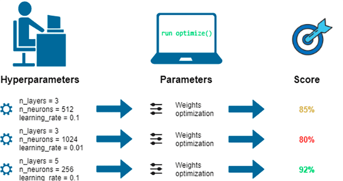Figure 1: Tuning deep neural network hyperparameters with scikit-learn (image source).

This tutorial on hyperparameter tuning for neural networks was inspired by a question I received by PyImageSearch reader, Abigail:

Hi, Adrian,

Thanks for all the tutorials on neural networks. I have some questions about choosing/building an architecture:

How do you ‘know’ the number of nodes to use in a given layer?

How do you choose a learning rate?

What is the optimal batch size?

How do you know how many epochs to train the network for?

If you could shed some light on that, I would really appreciate it.”

In general, there are three ways to set these values:

Do nothing (just guess): This is what many first-time machine learning practitioners do. They read a book, tutorial, or guide, see what other architectures use, and then simply copy and paste into their own code. Sometimes this works, sometimes it doesn’t — but in nearly all situations, you’re leaving some accuracy on the table by not tuning your hyperparameters.
Rely on your experience: Training a deep neural network is part art, part science. Once you’ve trained 100s or 1000s of neural networks, you start to develop a sixth sense as to what works and what doesn’t. The problem is that it takes a long time to get to this level (and there, of course, will be situations where your gut instinct is simply incorrect).
Tune your hyperparameters algorithmically: This is your foolproof method to finding optimal hyperparameters. Yes, it’s a bit time-consuming due to the need to run 100s or even 1000s of trials, but you’re guaranteed to get some improvement here.

Today, we’ll learn how to tune the following hyperparameters to a neural network:

The number of nodes in layers
The learning rate
Dropout rate
Batch size
Epochs to train for

We’ll accomplish this task by:

Implementing a basic neural network architecture
Defining the hyperparameter space to search over
Instantiating an instance of KerasClassifier from the tensorflow.keras.wrappers.scikit_learn submodule
Running a randomized search via scikit-learn’s RandomizedSearchCV class overtop the hyperparameters and model architecture

By the end of this guide, we’ll have boosted our accuracy from 78.59% (no hyperparameter tuning) up to 98.28% accuracy (with hyperparameter tuning).

Configuring your development environment

This tutorial on hyperparameter tuning requires Keras and TensorFlow. If you intend to follow this tutorial, I suggest you take the time to configure your deep learning development environment.

You can utilize either of these two guides to install TensorFlow and Keras on your system:

Either tutorial will help configure your system with all the necessary software for this blog post in a convenient Python virtual environment.

Having problems configuring your development environment?

Figure 2: Having trouble configuring your dev environment? Want access to pre-configured Jupyter Notebooks running on Google Colab? Be sure to join PyImageSearch University — you’ll be up and running with this tutorial in a matter of minutes.

All that said, are you:

Short on time?
Learning on your employer’s administratively locked system?
Wanting to skip the hassle of fighting with the command line, package managers, and virtual environments?
Ready to run the code right now on your Windows, macOS, or Linux systems?

Then join PyImageSearch University today!

Gain access to Jupyter Notebooks for this tutorial and other PyImageSearch guides that are pre-configured to run on Google Colab’s ecosystem right in your web browser! No installation required.

And best of all, these Jupyter Notebooks will run on Windows, macOS, and Linux!

Project structure

Before we implement any code, let’s first ensure we understand our project directory structure.

Be sure to access the “Downloads” section of this guide to retrieve the source code.

You’ll then be presented with the following directory structure:

$ tree . --dirsfirst
.
├── pyimagesearch
│   └── mlp.py
├── random_search_mlp.py
└── train.py

1 directory, 3 files

Inside the pyimagesearch module, we have a single file, mlp.py. This script contains get_mlp_model, which accepts several parameters and then builds a multi-layer perceptron (MLP) architecture. The parameters it accepts will be set by our hyperparameter tuning algorithm, thereby allowing us to tune the internal parameters of the network programmatically.

To establish a baseline with no hyperparameter tuning, we’ll use the train.py script to create an instance of our MLP and then train it on the MNIST digits dataset.

Once our baseline has been established, we’ll perform a random hyperparameter search via random_search_mlp.py.

As the results section of this tutorial will show, a hyperparameter search results in a massive jump in accuracy — an $\pmb\approx$ $\pmb\approx$ 20% increase!

Implementing our basic feedforward neural network

To tune the hyperparameters of a neural network, we first need to define the model architecture. Inside the model architecture, we’ll include variables for the number of nodes in a given layer and dropout rate.

We’ll also include the learning rate for the optimizer itself.

This model, once constructed, will be returned to the hyperparameter tuner. The tuner will then fit the neural network on our training data, evaluate it, and return the score.

After all trials are complete, the hyperparameter tuner will tell us which hyperparameters provided the best accuracy.

But it all starts with implementing the model architecture itself. Open the mlp.py file in the pyimagesearch module, and let’s get to work:

# import the necessary packages
from tensorflow.keras.models import Sequential
from tensorflow.keras.layers import Flatten
from tensorflow.keras.layers import Dropout
from tensorflow.keras.layers import Dense
from tensorflow.keras.optimizers import Adam

Lines 2-6 import our required Python packages. These are all fairly standard imports for building a basic feedforward neural network. If you need to learn the basics of building neural networks with Keras/TensorFlow, I recommend reading this tutorial.

Let’s now define our get_mlp_model function, which is responsible for accepting the hyperparameters we want to test, constructing the neural network, and returning it:

def get_mlp_model(hiddenLayerOne=784, hiddenLayerTwo=256,
	dropout=0.2, learnRate=0.01):
	# initialize a sequential model and add layer to flatten the
	# input data
	model = Sequential()
	model.add(Flatten())

Our get_mlp_model accepts four parameters, including:

hiddenLayerOne: Number of nodes in the first fully connected layer
hiddenLayerTwo: Number of nodes in the second fully connected layer
dropout: Dropout rate between the fully connected layers (useful to reduce overfitting)
learnRate: Learning rate for the Adam optimizer

Lines 12-13 start building the model architecture.

Let’s continue building the architecture in the following code block:

	# add two stacks of FC => RELU => DROPOUT
	model.add(Dense(hiddenLayerOne, activation="relu",
		input_shape=(784,)))
	model.add(Dropout(dropout))
	model.add(Dense(hiddenLayerTwo, activation="relu"))
	model.add(Dropout(dropout))

	# add a softmax layer on top
	model.add(Dense(10, activation="softmax"))

	# compile the model
	model.compile(
		optimizer=Adam(learning_rate=learnRate),
		loss="sparse_categorical_crossentropy",
		metrics=["accuracy"])

	# return compiled model
	return model

Lines 16-20 define two stacks of FC => RELU => DROPOUT layers.

Notice that we’re utilizing our hiddenLayerOne, hiddenLayerTwo, and dropout layers when building the architecture. Encoding each of these values as variables allows us to supply different values to the get_mlp_model when performing a hyperparameter search. Doing so is the “magic” in how scikit-learn can tune hyperparameters to a Keras/TensorFlow model.

Line 23 adds a softmax classifier on top of our final FC Layer.

We then compile the model using the Adam optimizer and the specified learnRate (which will be tuned via our hyperparameter search).

The resulting model is returned to the calling function on Line 32.

Creating our basic training script (no hyperparameter tuning)

Before we perform a hyperparameter search, let’s first obtain a baseline with no hyperparameter tuning. Doing so will give us a baseline accuracy score for us to beat.

Open the train.py file in your project directory structure, and let’s get to work:

# import tensorflow and fix the random seed for better reproducibility
import tensorflow as tf
tf.random.set_seed(42)

# import the necessary packages
from pyimagesearch.mlp import get_mlp_model
from tensorflow.keras.datasets import mnist

Lines 2 and 3 import the TensorFlow library and fixes the random seed. Fixing the random seed helps (but does not necessarily guarantee) better reproducibility.

Keep in mind that neural networks are stochastic algorithms, implying there is a bit of randomness involved, particularly in:

Layer initialization (nodes in a neural network are initialized from a random distribution)
Training and testing set splits
Any randomness injected during data batching

Using a fixed seed helps improve reproducibility by ensuring at least the layer initialization randomness is consistent (ideally).

From there, we load the MNIST dataset:

# load the MNIST dataset
print("[INFO] downloading MNIST...")
((trainData, trainLabels), (testData, testLabels)) = mnist.load_data()

# scale data to the range of [0, 1]
trainData = trainData.astype("float32") / 255.0
testData = testData.astype("float32") / 255.0

If this is the first time you’ve used Keras/TensorFlow, then the MNIST dataset will be downloaded and cached to your disk.

We then scale the pixel intensities in the training and testing images from the range [0, 255] to [0, 1], a common preprocessing technique when working with neural networks.

Let’s now train our basic feedforward network:

# initialize our model with the default hyperparameter values
print("[INFO] initializing model...")
model = get_mlp_model()

# train the network (i.e., no hyperparameter tuning)
print("[INFO] training model...")
H = model.fit(x=trainData, y=trainLabels,
	validation_data=(testData, testLabels),
	batch_size=8,
	epochs=20)

# make predictions on the test set and evaluate it
print("[INFO] evaluating network...")
accuracy = model.evaluate(testData, testLabels)[1]
print("accuracy: {:.2f}%".format(accuracy * 100))

Line 19 makes a call to the get_mlp_model function to build our neural network with the default options (we’ll later tune the learning rate, dropout rate, and number of hidden layer nodes via a hyperparameter search).

Lines 23-26 train our neural network.

We then evaluate the accuracy of the model on our testing set via Lines 30 and 31.

This accuracy will serve as the baseline we need to beat when performing a hyperparameter search.

Obtaining baseline accuracy

Before we can tune the hyperparameters to our network, let’s first obtain a baseline with our “default” configuration (i.e., hyperparameters, that based on our experience, we think will yield good accuracy).

Start by accessing the “Downloads” section of this tutorial to retrieve the source code.

From there, open a shell and execute the following command:

$ time python train.py
Epoch 1/20
7500/7500 [==============================] - 18s 2ms/step - loss: 0.8881 - accuracy: 0.7778 - val_loss: 0.4856 - val_accuracy: 0.9023
Epoch 2/20
7500/7500 [==============================] - 17s 2ms/step - loss: 0.6887 - accuracy: 0.8426 - val_loss: 0.4591 - val_accuracy: 0.8658
Epoch 3/20
7500/7500 [==============================] - 17s 2ms/step - loss: 0.6455 - accuracy: 0.8466 - val_loss: 0.4536 - val_accuracy: 0.8960
...
Epoch 18/20
7500/7500 [==============================] - 19s 2ms/step - loss: 0.8592 - accuracy: 0.7931 - val_loss: 0.6860 - val_accuracy: 0.8776
Epoch 19/20
7500/7500 [==============================] - 17s 2ms/step - loss: 0.9226 - accuracy: 0.7876 - val_loss: 0.9510 - val_accuracy: 0.8452
Epoch 20/20
7500/7500 [==============================] - 17s 2ms/step - loss: 0.9810 - accuracy: 0.7825 - val_loss: 0.8294 - val_accuracy: 0.7859
[INFO] evaluating network...
313/313 [==============================] - 1s 2ms/step - loss: 0.8294 - accuracy: 0.7859
accuracy: 78.59%

real	5m48.320s
user	19m53.908s
sys	2m25.608s

Using the default hyperparameters from our implementation with no hyperparameter tuning, we could reach 78.59% accuracy.

Now that we have our baseline, we can treat to beat it — and as you’ll see, applying hyperparameter tuning blows this result out of the water!

Implementing our Keras/TensorFlow hyperparameter tuning script

Let’s learn how we can use scikit-learn to tune the hyperparameters to a Keras/TensorFlow model.

We start with our imports:

# import tensorflow and fix the random seed for better reproducibility
import tensorflow as tf
tf.random.set_seed(42)

# import the necessary packages
from pyimagesearch.mlp import get_mlp_model
from tensorflow.keras.wrappers.scikit_learn import KerasClassifier
from sklearn.model_selection import RandomizedSearchCV
from tensorflow.keras.datasets import mnist

Again, Lines 2-3 import TensorFlow and fix our random seed for better reproducibility.

Lines 6-9 import our required Python packages, including:

get_mlp_model: Accepts several hyperparameters and constructs a neural network based on them
KerasClassifier: Takes a Keras/TensorFlow model and wraps it in a manner such that it’s compatible with scikit-learn functions (such as scikit-learn’s hyperparameter tuning functions)
RandomizedSearchCV: scikit-learn’s implementation of a random hyperparameter search (see this tutorial if you are unfamiliar with a randomized hyperparameter tuning algorithm)
mnist: The MNIST dataset

We can then proceed to load the MNIST dataset from disk and preprocess it:

# load the MNIST dataset
print("[INFO] downloading MNIST...")
((trainData, trainLabels), (testData, testLabels)) = mnist.load_data()

# scale data to the range of [0, 1]
trainData = trainData.astype("float32") / 255.0
testData = testData.astype("float32") / 255.0

It’s now time to construct our KerasClassifier object such that we can build a model with get_mlp_model and then tune the hyperparameters with RandomizedSearchCV:

# wrap our model into a scikit-learn compatible classifier
print("[INFO] initializing model...")
model = KerasClassifier(build_fn=get_mlp_model, verbose=0)

# define a grid of the hyperparameter search space
hiddenLayerOne = [256, 512, 784]
hiddenLayerTwo = [128, 256, 512]
learnRate = [1e-2, 1e-3, 1e-4]
dropout = [0.3, 0.4, 0.5]
batchSize = [4, 8, 16, 32]
epochs = [10, 20, 30, 40]

# create a dictionary from the hyperparameter grid
grid = dict(
	hiddenLayerOne=hiddenLayerOne,
	learnRate=learnRate,
	hiddenLayerTwo=hiddenLayerTwo,
	dropout=dropout,
	batch_size=batchSize,
	epochs=epochs
)

Line 21 instantiates our KerasClassifier object. We pass in our get_mlp_model function, telling Keras/TensorFlow that the get_mlp_model function is responsible for building and constructing the model architecture.

Next, Lines 24-39 define our hyperparameter search space. We’ll be tuning:

The number of nodes in the first fully connected layer
The number of nodes in the second fully connected layer
Our learning rate
Dropout rate
Batch size
Number of epochs to train for

The hyperparameters are then added to a Python dictionary named grid.

Note that the keys to the dictionary are the same names of the variables inside get_mlp_model. Furthermore, the batch_size and epochs variables are the same variables you would supply when calling model.fit with Keras/TensorFlow.

This naming convention is by design and is required when you construct a Keras/TensorFlow model and seek to tune the hyperparameters with scikit-learn.

With our grid of hyperparameters defined we can kick off the hyperparameter tuning process:

# initialize a random search with a 3-fold cross-validation and then
# start the hyperparameter search process
print("[INFO] performing random search...")
searcher = RandomizedSearchCV(estimator=model, n_jobs=-1, cv=3,
	param_distributions=grid, scoring="accuracy")
searchResults = searcher.fit(trainData, trainLabels)

# summarize grid search information
bestScore = searchResults.best_score_
bestParams = searchResults.best_params_
print("[INFO] best score is {:.2f} using {}".format(bestScore,
	bestParams))

Lines 44 and 45 initialize our searcher. We pass in the model, the number of parallel jobs to run a value of -1 tells scikit-learn to use all cores/processors on your machine, the number of cross-validation folds, the hyperparameter grid, and the metric we want to monitor.

From there, a call to fit of the searcher starts the hyperparameter tuning process.

Once the search is complete, we obtain the bestScore and bestParams found during the search, displaying both of them on our terminal (Lines 49-52).

The final step is to obtain the bestModel and evaluate it:

# extract the best model, make predictions on our data, and show a
# classification report
print("[INFO] evaluating the best model...")
bestModel = searchResults.best_estimator_
accuracy = bestModel.score(testData, testLabels)
print("accuracy: {:.2f}%".format(accuracy * 100))

Line 57 grabs the best_estimator_ from the randomized search.

We then evaluate the best model on our testing data and display the accuracy on our screen (Lines 58 and 59).

Tuning Keras/TensorFlow hyperparameters with scikit-learn results

Let’s see how our Keras/TensorFlow hyperparameter tuning script performs.

Access the “Downloads” section of this tutorial to retrieve the source code.

From there, you can execute the following command:

$ time python random_search_mlp.py
[INFO] downloading MNIST...
[INFO] initializing model...
[INFO] performing random search...
[INFO] best score is 0.98 using {'learnRate': 0.001, 'hiddenLayerTwo': 256, 'hiddenLayerOne': 256, 'epochs': 40, 'dropout': 0.4, 'batch_size': 32}
[INFO] evaluating the best model...
accuracy: 98.28%

real    22m52.748s
user    151m26.056s
sys     12m21.016s

The random_search_mlp.py script took $\approx$ $\approx$ 4x longer to run than our basic no hyperparameter tuning script ( $\approx$ $\approx$ 23m versus $\approx$ $\approx$ 6m, respectively) — but that extra time is well worth it as the difference in accuracy is tremendous.

Without any hyperparameter tuning, we only obtained 78.59% accuracy. But by applying a randomized hyperparameter search with scikit-learn, we were able to boost our accuracy up to 98.28%!

That is a tremendous boost in accuracy — and one that would not have been possible without applying a dedicated hyperparameter search.

What’s next? I recommend PyImageSearch University.

Course information:
69 total classes • 73 hours of on-demand code walkthrough videos • Last updated: February 2023

★★★★★

4.84 (128 Ratings) • 15,800+ Students Enrolled

I strongly believe that if you had the right teacher you could master computer vision and deep learning.

Do you think learning computer vision and deep learning has to be time-consuming, overwhelming, and complicated? Or has to involve complex mathematics and equations? Or requires a degree in computer science?

That’s not the case.

All you need to master computer vision and deep learning is for someone to explain things to you in simple, intuitive terms. And that’s exactly what I do. My mission is to change education and how complex Artificial Intelligence topics are taught.

If you’re serious about learning computer vision, your next stop should be PyImageSearch University, the most comprehensive computer vision, deep learning, and OpenCV course online today. Here you’ll learn how to successfully and confidently apply computer vision to your work, research, and projects. Join me in computer vision mastery.

Inside PyImageSearch University you’ll find:

&check; 69 courses on essential computer vision, deep learning, and OpenCV topics
&check; 69 Certificates of Completion
&check; 73 hours of on-demand video
&check; Brand new courses released regularly, ensuring you can keep up with state-of-the-art techniques
&check; Pre-configured Jupyter Notebooks in Google Colab
&check; Run all code examples in your web browser — works on Windows, macOS, and Linux (no dev environment configuration required!)
&check; Access to centralized code repos for all 500+ tutorials on PyImageSearch
&check; Easy one-click downloads for code, datasets, pre-trained models, etc.
&check; Access on mobile, laptop, desktop, etc.

Click here to join PyImageSearch University

Summary

In this tutorial, you learned how to tune hyperparameters to a deep neural network using scikit-learn, Keras, and TensorFlow.

By using Keras/TensorFlow’s KerasClassifier implementation, we were able to wrap our model architecture such that it became compatible with scikit-learn’s RandomizedSearchCV class.

From there, we:

Randomly sampled from our hyperparameter space
Trained our neural network (with cross-validation) on the current set of hyperparameters
Evaluated the model’s performance

At the end of trials, we obtained the best hyperparameters from the randomized search, trained the final model, and evaluated accuracy:

Without hyperparameter tuning, we were only able to obtain 78.59% accuracy
But with hyperparameter tuning, we hit 98.28% accuracy

As you can see, tuning hyperparameters to a neural network can make a huge difference in accuracy … and this was only on the simple MNIST dataset. Imagine what it can do for your more complex, real-world datasets!

To download the source code to this post (and be notified when future tutorials are published here on PyImageSearch), simply enter your email address in the form below!

Download the Source Code and FREE 17-page Resource Guide

Enter your email address below to get a .zip of the code and a FREE 17-page Resource Guide on Computer Vision, OpenCV, and Deep Learning. Inside you’ll find my hand-picked tutorials, books, courses, and libraries to help you master CV and DL!