Feedforward Neural Networks | Brilliant Math & Science Wiki

The simplest type of feedforward neural network is the perceptron, a feedforward neural network with no hidden units. Thus, a perceptron has only an input layer and an output layer. The output units are computed directly from the sum of the product of their weights with the corresponding input units, plus some bias.

Historically, the perceptron’s output has been binary, meaning it outputs a value of \(0\) or \(1\). This is achieved by passing the aforementioned product sum into the step function \(H(x)\). This is defined as

\(H(x) = \begin{cases}
1 && \mbox{if }\ x \ge 0 \\
0 && \mbox{if }\ x \lt 0.
\end{cases}\)

For a binary perceptron with \(n\)-dimensional input \(\vec{x}\), \(n\)-dimensional weight vector \(\vec{w}\), and bias \(b\), the \(1\)-dimensional output \(o\) is

\(o = \begin{cases}
1 && \mbox{if }\ \vec{w} \cdot \vec{x} + b \ge 0 \\
0 && \mbox{if }\ \vec{w} \cdot \vec{x} + b \lt 0.
\end{cases}\)

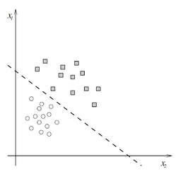
Since the perceptron divides the input space into two classes, \(0\) and \(1\), depending on the values of \(\vec{w}\) and \(b,\) it is known as a linear classifier. The diagram to the right displays one such linear classifier. The line separating the two classes is known as the classification boundary or decision boundary. In the case of a two-dimensional input (as in the diagram) it is a line, while in higher dimensions this boundary is a hyperplane. The weight vector \(\vec{w}\) defines the slope of the classification boundary while the bias \(b\) defines the intercept.

More general single-layer peceptrons can use activation functions other than the step function \(H(x)\). Typical choices are the identity function \(f(x) = x,\) the sigmoid function \(\sigma(x) = \left(1 + e^{-x}\right)^{-1},\) and the hyperbolic tangent \(\tanh (x) = \frac{e^{x} + e^{-x}}{e^{x} – e^{-x}}.\) Use of any of these functions ensures the output is a continuous number (as opposed to binary), and thus not every activation function yields a linear classifier.

Generally speaking, a perceptron with activation function \(g(x)\) has output

\[o = g(\vec{w} \cdot \vec{x} + b).\]

In order for a perceptron to learn to correctly classify a set of input-output pairs \((\vec{x}, y)\), it has to adjust the weights \(\vec{w}\) and bias \(b\) in order to learn a good classification boundary. The figure below shows many possible classification boundaries, the best of which is the boundary labeled \(H_2\). If the perceptron uses an activation function other than the step function (e.g. the sigmoid function), then the weights and bias should be adjusted so that the output \(o\) is close to the true label \(y\).

Error Function

Typically, the learning process requires the definition of an error function \(E\) that quantifies the difference between the computed output of the perceptron \(o\) and the true value \(y\) for an input \(\vec{x}\) over a set of multiple input-output pairs \((\vec{x}, y)\). Historically, this error function is the mean squared error (MSE), defined for a set of \(N\) input-output pairs \(X = \{(\vec{x_1}, y_1), \dots, (\vec{x_N}, y_N)\}\) as

\[E(X) = \frac{1}{2N} \sum_{i=1}^N \left(o_i – y_i\right)^2 = \frac{1}{2N} \sum_{i=1}^N \left(g(\vec{w} \cdot \vec{x_i} + b) – y_i\right)^2,\]

where \(o_i\) denotes the output of the perceptron on input \(\vec{x_i}\) with activation function \(g\). The factor of \(\frac{1}{2}\) is included in order to simplify the calculation of the derivative later. Thus, \(E(X) = 0\) when \(o_i = y_i\) for all input-output pairs \((\vec{x_i}, y_i)\) in \(X\), so a natural objective is to attempt to change \(\vec{w}\) and \(b\) such that \(E(X)\) is as close to zero as possible. Thus, minimizing \(E(X)\) with respect to \(\vec{w}\) and \(b\) should yield a good classification boundary.

Delta Rule

\(E(X)\) is typically minimized using gradient descent, meaning the perceptron adjusts \(\vec{w}\) and \(b\) in the direction of the negative gradient of the error function. Gradient descent works for any error function, not just the mean squared error. This iterative process reduces the value of the error function until it converges on a value, usually a local minimum. The values of \(\vec{w}\) and \(b\) are typically set randomly and then updated using gradient descent. If the random initializations of \(\vec{w}\) and \(b\) are denoted \(\vec{w_0}\) and \(b_0\), respectively, then gradient descent updates \(\vec{w}\) and \(b\) according to the equations

\[\vec{w_{i+1}} = \vec{w_i } – \alpha \frac{\partial E(X)}{\partial \vec{w_i}}\\
b_{i+1} = b_i – \alpha \frac{\partial E(X)}{\partial b_i},\]

where \(\vec{w_i}\) and \(b_i\) are the values of \(\vec{w}\) and \(b\) after the \(i^\text{th}\) iteration of gradient descent, and \(\frac{\partial f}{\partial x}\) is the partial derivative of \(f\) with respect to \(x\). \(\alpha\) is known as the learning rate, which controls the step size gradient descent takes each iteration, typically chosen to be a small value, e.g. \(\alpha = 0.01.\) Values of \(\alpha\) that are too large cause learning to be suboptimal (by failing to converge), while values of \(\alpha\) that are too small make learning slow (by taking too long to converge).

The weight delta \(\Delta \vec{w} = \vec{w_{i+1}} – \vec{w_{i}}\) and bias delta \(\Delta b = b_{i+1} – b_i\) are calculated using the delta rule. The delta rule is a special case of backpropagation for single-layer perceptrons, and is used to calculate the updates (or deltas) of the perceptron parameters. The delta rule can be derived by consistent application of the chain rule and power rule for calculating the partial derivatives \(\frac{\partial E(X)}{\partial \vec{w_i}}\) and \(\frac{\partial E(X)}{\partial b_i}.\) For a perceptron with a mean squared error function and activation function \(g\), the delta rules for the weight vector \(\vec{w}\) and bias \(b\) are

\[\Delta \vec{w} = \frac{1}{N} \sum_{i=1}^N \alpha (y_i – o_i) g'(h_i) \vec{x_i}\\\\
\Delta b = \frac{1}{N} \sum_{i=1}^N \alpha (y_i – o_i) g'(h_i),\]

where \(o_i = g(\vec{w} \cdot \vec{x_i} + b)\) and \(h_i = \vec{w} \cdot \vec{x_i} + b\). Note that the presence of \(\vec{x_i}\) on the right side of the delta rule for \(\vec{w}\) implies that the weight vector’s update delta is also a vector, which is expected.

Training the Perceptron

Thus, given a set of \(N\) input-output pairs \(X = \left\{\big(\vec{x_1}, y_1\big), \ldots, \big(\vec{x_N}, y_N\big)\right\},\) learning consists of iteratively updating the values of \(\vec{w}\) and \(b\) according to the delta rules. This consists of two distinct computational phases:

1. Calculate the forward values. That is, for \(X = \left\{\big(\vec{x_1}, y_1\big), \ldots, \big(\vec{x_N}, y_N\big)\right\},\) calculate \(h_i\) and \(o_i\) for all \(\vec{x_i}\).
2. Calculate the backward values. Using the partial derivatives of the error function, update the weight vector and bias according to gradient descent. Specifically, use the delta rules and the values calculated in the forward phase to calculate the deltas for each.

The backward phase is so named because in multi-layer perceptrons there is no simple delta rule, so calculation of the partial derivatives proceeds backwards from the error between the target output and actual output \(y_i – o_i\) (this is where backpropagation gets its name). In a single-layer perceptron, there is no backward flow of information (there is only one “layer” of parameters), but the naming convention applies all the same.

Once the backward values are computed, they may be used to update the values of the weight vector \(\vec{w}\) and bias \(b\). The process repeats until the error function \(E(X)\) converges. Once the error function has converged, the weight vector \(\vec{w}\) and bias \(b\) can be fixed, and the forward phase used to calculate predicted values \(o\) of the true output \(y\) for any input \(x\). If the perceptron has learned the underlying function mapping inputs to outputs \(\big(\)i.e. not just remembered every pair of \((\vec{x_i}, y_i)\big),\) it will even predict the correct values for input-output pairs it was not trained on, known as generalization. Ultimately, generalization is the primary goal of supervised learning, since it is desirable and a practical necessity to learn an unknown function based on a small sample of the set of all possible input-output pairs.