Build a neural network in 7 steps

In this tutorial, we build a neural network that approximates a function defined by a set of data points.

The data for this application can be obtained from the
data.csv file.

To solve this application, follow the next steps:

1. Create approximation model

Open Neural Designer.
The start page is shown.

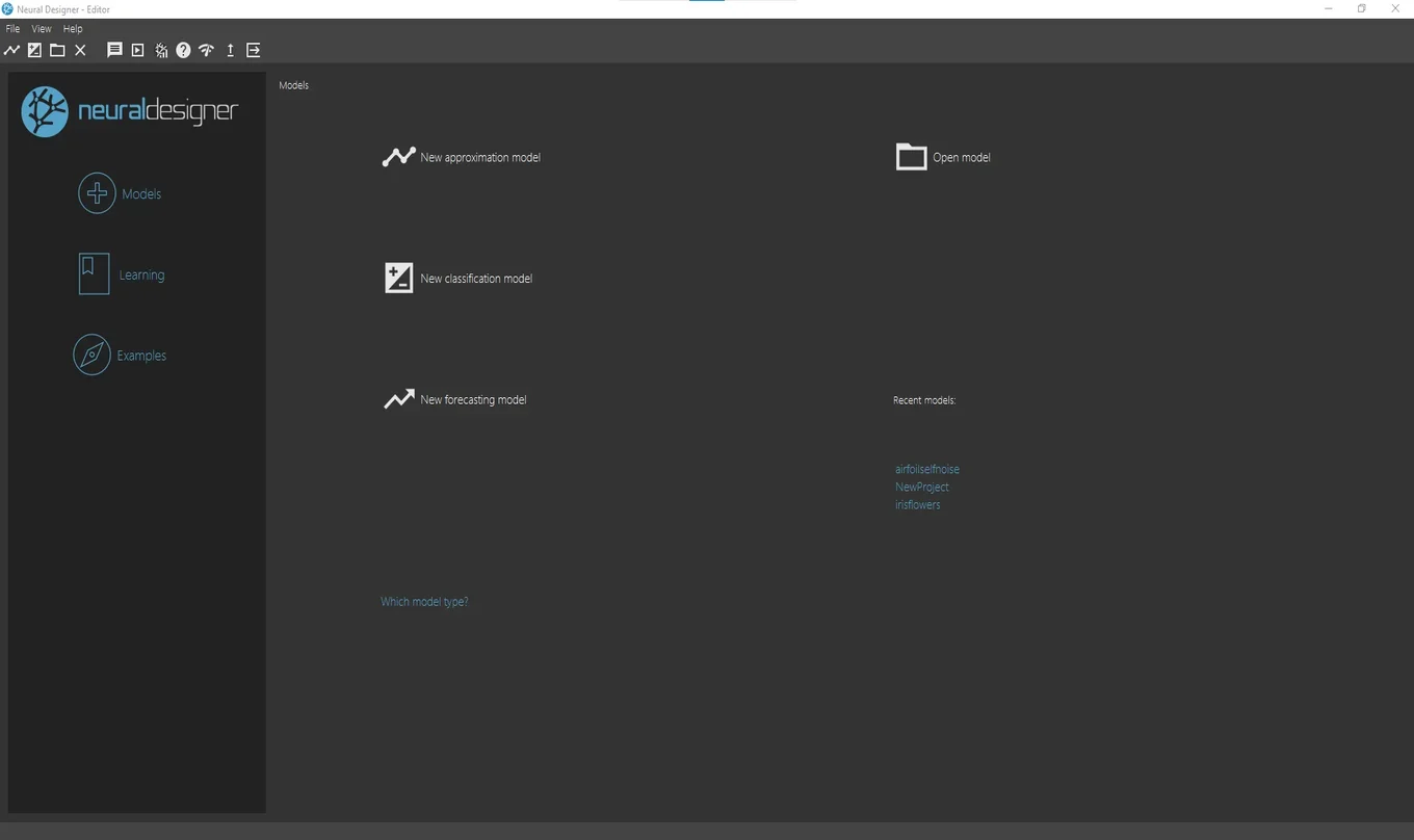
Click on the button New approximation model.
Save the project file in the same folder as the data file.
The main view of Neural Designer is shown.

2. Configure data set

In the Data set page, click on the Import data file button.
A file chooser dialogue will appear.
Select the file data.csv.
Click on the Finish button.
The program loads the data and sets the default configuration.

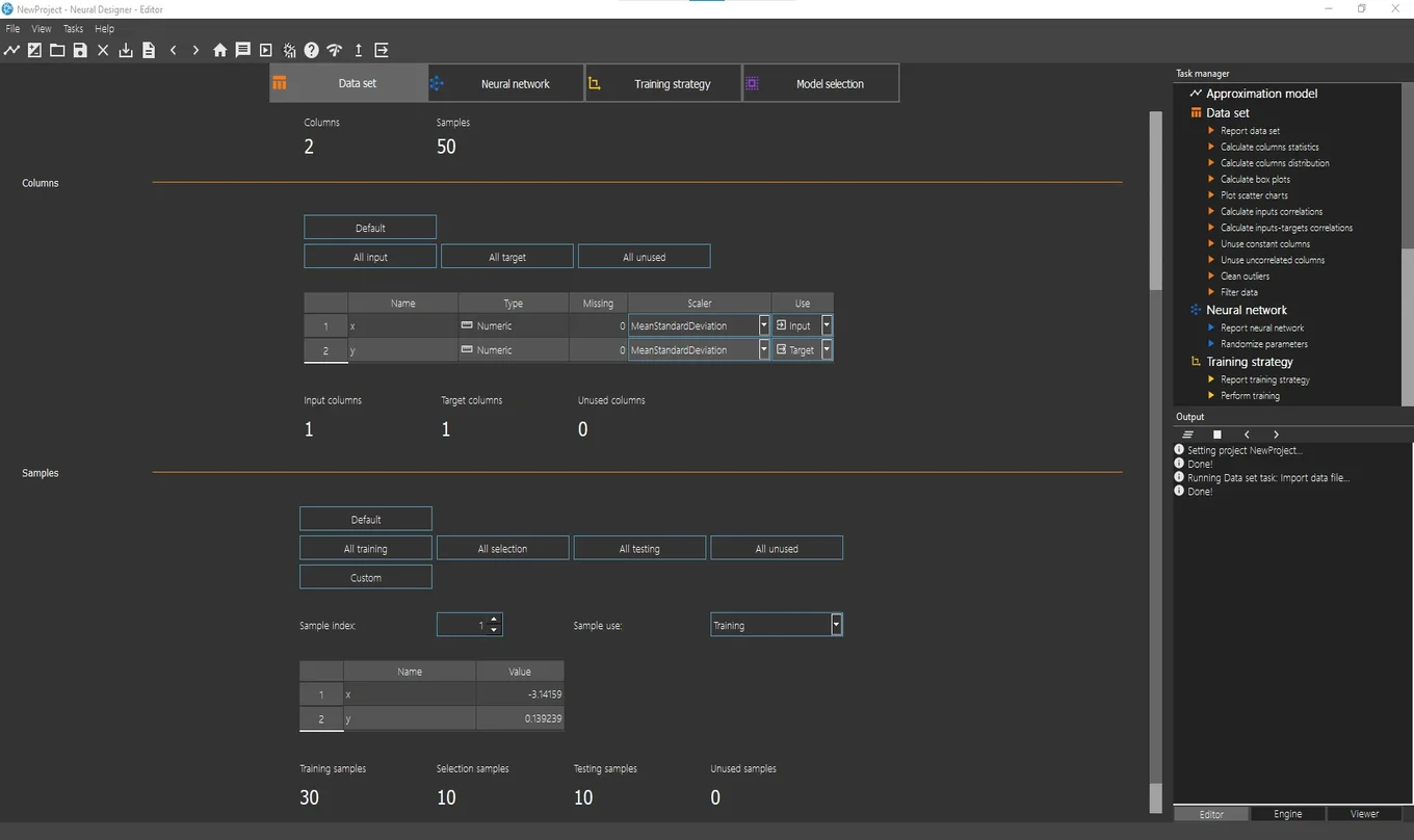
This data set has 2 variables and 50 samples.

We define the use of the variables:
-The first column represents the independent variable, or input variable, x.
-The second column represents the dependent variable, or target variable, y.
We leave that default values.

Then we define the use of the instances:
-60% of the data is used for training.
-20% of the data is used for selection.
-20% of the data is used for testing.
We leave that default values.

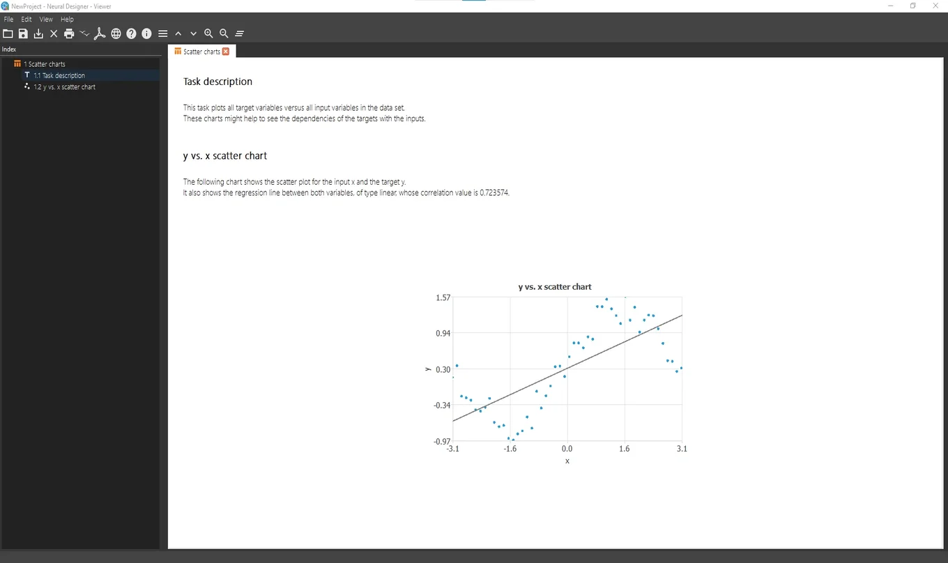
Once the data set is configured, we can run some dataset analysis related tasks.
For instance, in the Task Manager, click on Data set> Plot scatter chart.
The viewer window will appear with a chart of the data.
As we can see, the shape of this data is a sinus function.

You can check the data quality by running different data set tasks.

3. Set network architecture

Click on the Neural network tab to configure the
approximation model.
The next screenshot shows this page.

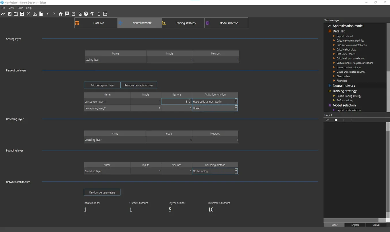
The Perceptron layers section is the most important one here.
By default, the number of layers is 2 (hidden layer and output layer).
By default, the hidden layer has 3 neurons with a hyperbolic tangent activation function.
As we have 1 target (y), the output layer must have 1 neuron. The default activation function here is the linear activation function.
We leave that default values.

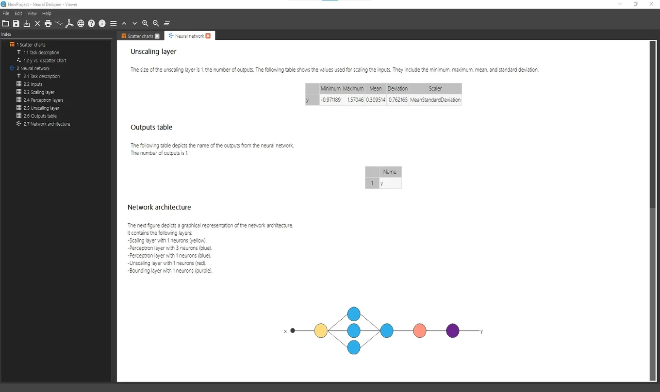
To visualize the
network architecture,
click on Task manager> Neural network> Report neural network.
The viewer window will appear with a graph of the network architecture.

4. Train neural network

In the Training strategy
page, the information about the error method
and the optimization algorithm is set.
The next figure shows this page.

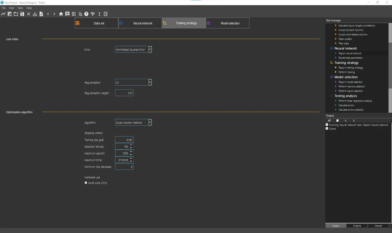
The normalized squared error
is the default error method. A regularization term
is also added here.
The quasi-Newton method
is the default optimization algorithm.
We leave that default values.

The most important task is the so-called Perform training, which appears in the Task manager’s list of Training strategy tasks.
Running that task, the optimization algorithm
minimizes the loss index,
i.e., makes the neural network to fit the data set.
The following figure shows the results from the Perform training task in the Viewer window.

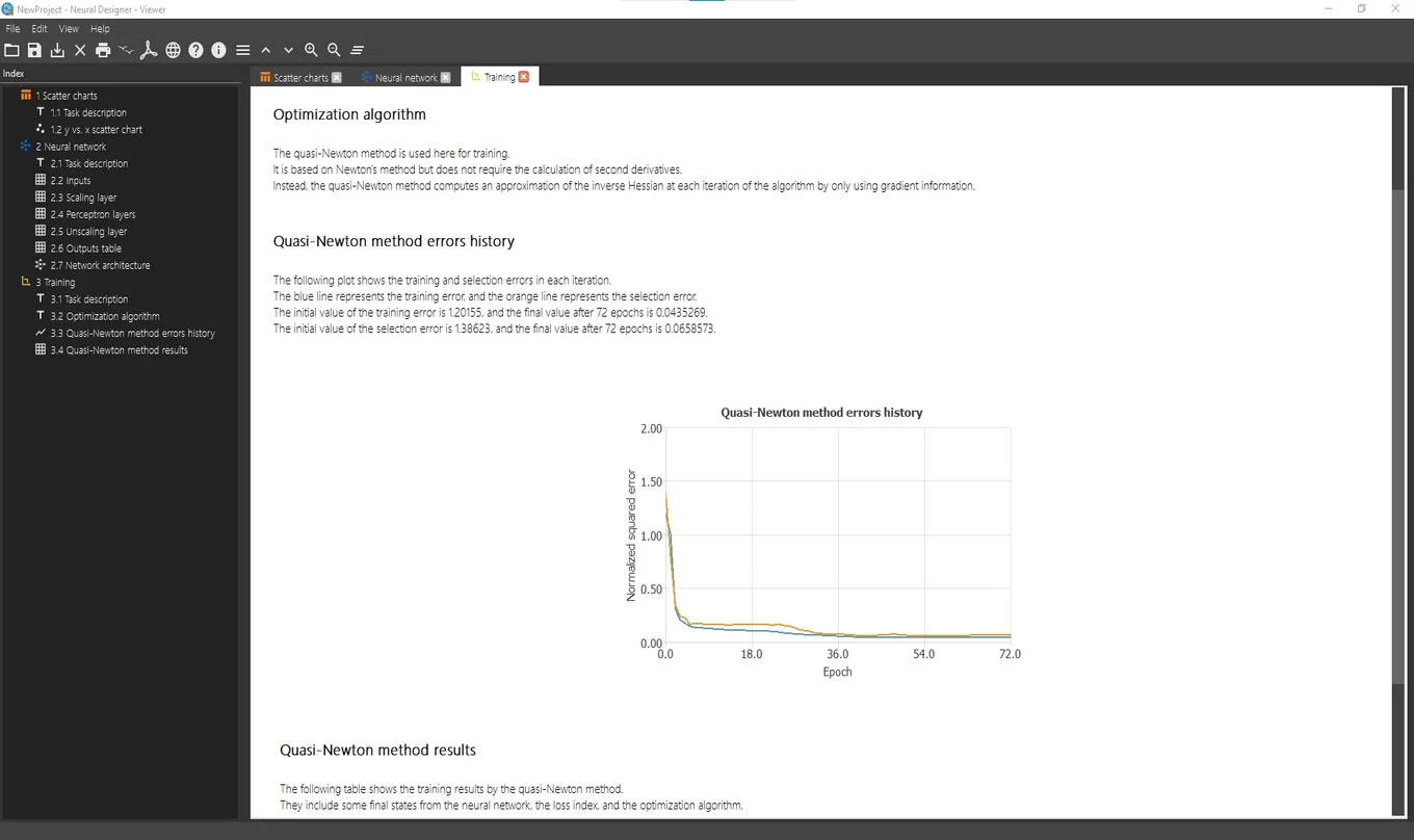
The figure above shows the training results.
It displays how both the training (blue) and selection (orange) errors decrease during the training process.

5. Improve generalization performance

The model selection tab shows the options that allow configuring the model selection process.
The next image shows the content of this page.

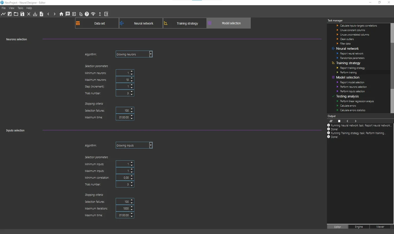
Growing neurons
and growing inputs
are the default options for Neurons selection and Inputs selection, respectively.
Since there is only one input, Input selection will not be needed.
To perform the Neurons selection, double click on Task manager> Model selection> Perform neurons selection
We leave the default values.
The figure below shows the Viewer windows with the results of this task.

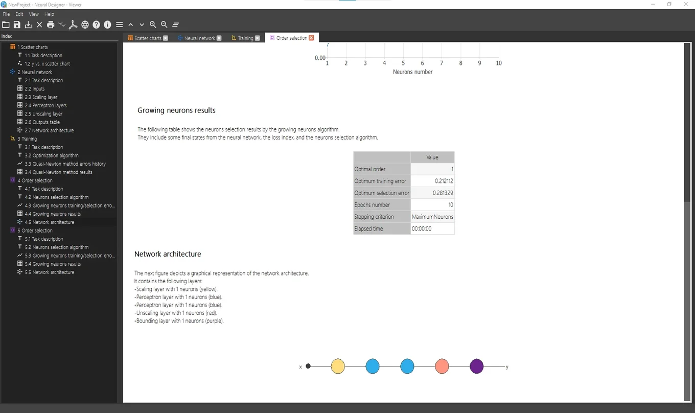
As we can see, an optimal network architecture
has been defined after performing the Neurons selection task.
This redefined neural network is already trained.

6. Test results

There are several tasks to test the model that has been previously trained. These tasks are grouped under
Testing analysis in the Task manager.

To test this model, double click on Task manager> Testing analysis> Perform linear regression analysis
The next figure shows the results of this task.

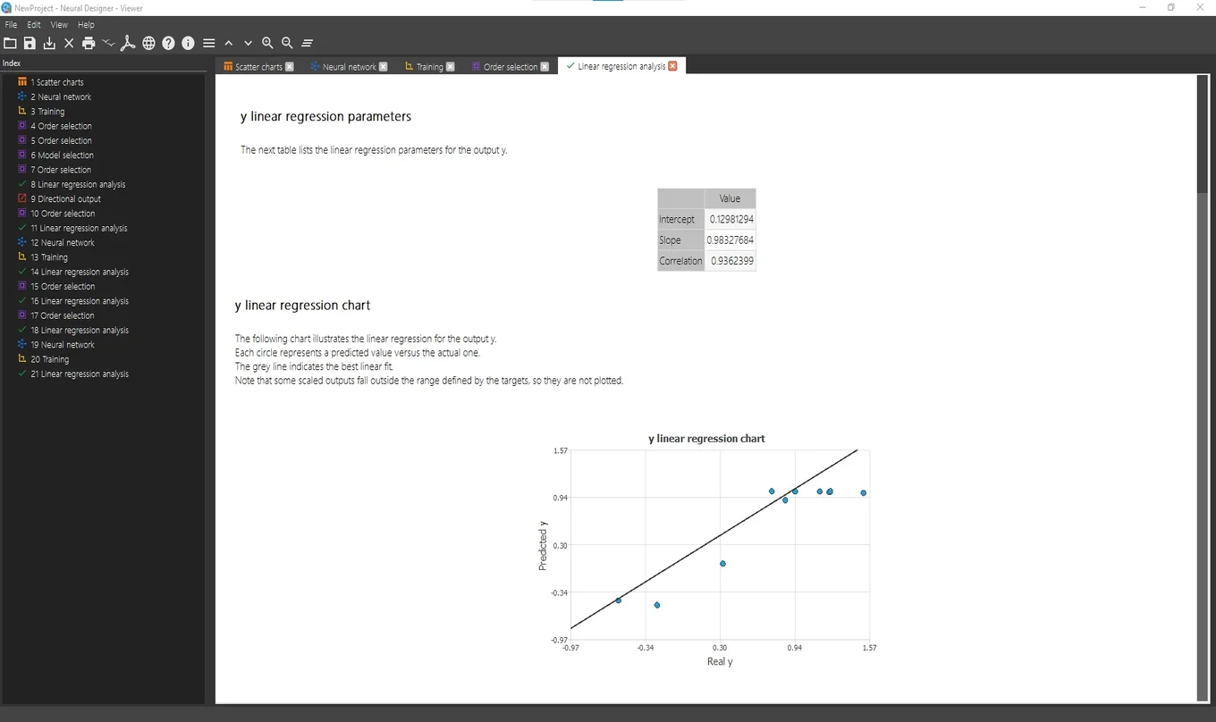
As we can observe in the table shown in the Viewer, the correlation is very close to 1, so we can say the model predicts well.

7. Deploy model

Once the model has been tested, it is ready to make predictions. The tasks for this purpose are found under
Model deployment in the Task manager.

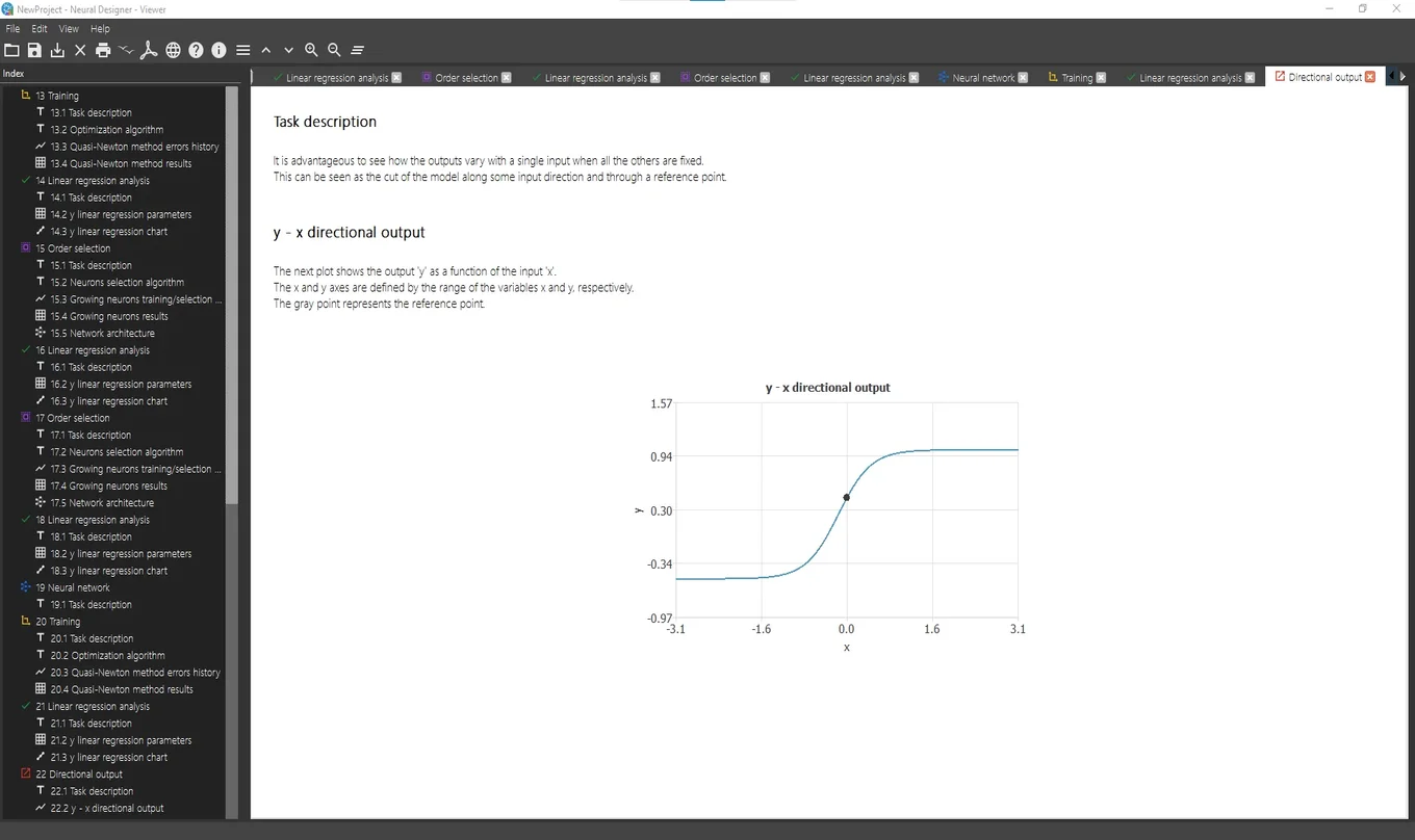
Double click on Task manager> Model deployment> Plot directional output
to see the output variation as a function of a single input.
The picture below shows the results after performing this task.

Model deployment tasks also include the option of writing the expression of the predictive model, in addition to exporting this expression to Python or C.
The Python code corresponding to this model is presented below.

import numpy as np

def scaling_layer(inputs):

	outputs = [None] * 1

	outputs[0] = inputs[0]*0.3183101416+0

	return outputs;


def perceptron_layer_0(inputs):

	combinations = [None] * 3

	combinations[0] = 0.0544993 +1.84365*inputs[0] 
	combinations[1] = -1.40552 -1.52111*inputs[0] 
	combinations[2] = 1.47629 -1.67521*inputs[0] 
	
	activations = [None] * 3

	activations[0] = np.tanh(combinations[0])
	activations[1] = np.tanh(combinations[1])
	activations[2] = np.tanh(combinations[2])

	return activations;


def perceptron_layer_1(inputs):

	combinations = [None] * 1

	combinations[0] = -0.094707 +1.89925*inputs[0] +1.47562*inputs[1] +1.54961*inputs[2] 
	
	activations = [None] * 1

	activations[0] = combinations[0]

	return activations;


def unscaling_layer(inputs):

	outputs = [None] * 1

	outputs[0] = inputs[0]*1.270824432+0.2996354103

	return outputs


def bounding_layer(inputs):

	outputs = [None] * 1

	outputs[0] = inputs[0]

	return outputs


def neural_network(inputs):

	outputs = [None] * len(inputs)

	outputs = scaling_layer(inputs)
	outputs = perceptron_layer_0(outputs)
	outputs = perceptron_layer_1(outputs)
	outputs = unscaling_layer(outputs)
	outputs = bounding_layer(outputs)

	return outputs;
     

To learn more, see the next example: