Build an Artificial Neural Network From Scratch: Part 1 – KDnuggets

This article focused on building an Artificial Neural Network using the Numpy Python library.

In my previous article Introduction to Artificial Neural Networks(ANN), we learned about various concepts related to ANN so I would recommend going through it before moving forward because here I’ll be focusing on the implementation part only. In this article series, we are going to build ANN from scratch using only the numpy Python library.

In this part-1, we will build a fairly easy ANN with just having 1 input layer and 1 output layer and no hidden layer.

In part-2, we will build ANN with 1 input layer, 1 hidden layer, and 1 output layer.

Why from scratch?

Well, there are many deep learning libraries(Keras, TensorFlow, PyTorch etc) that can be used to create a neural network in a few lines of code. However, if you really want to understand the in-depth working of a neural network, I suggest you learn how to code it from scratch using Python or any other programming language. So let’s get started.

Let’s create some random dataset:

 

In the above table, we have five columns: Person, X1, X2, X3, and Y. Here 1 refers to true and 0 refers to false. Our task is to create an artificial neural network that is capable of predicting the value of Y based on values of X1, X2 and X3.

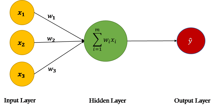
We will create an artificial neural network with one input layer and one output layer with no hidden layer. Before we start coding, let’s first let’s see how our neural network will execute in theory:

Theory of ANN

An artificial neural network is a supervised learning algorithm which means that we provide it the input data containing the independent variables and the output data that contains the dependent variable. For instance, in our example our independent variables are X1, X2 and X3. The dependent variable is Y.

In the beginning, the ANN makes some random predictions, these predictions are compared with the correct output and the error(the difference between the predicted values and the actual values) is calculated. The function that finds the difference between the actual value and the propagated values is called the cost function. The cost here refers to the error. Our objective is to minimize the cost function. Training a neural network basically refers to minimizing the cost function. We will see how we can perform this task.

A neural network executes in two phases: Feed Forward phase and Back Propagation phase. Let us discuss both these steps in detail.

 

Feed Forward

 

 

In the feed-forward phase of ANN, predictions are made based on the values in the input nodes and the weights. If you look at the neural network in the above figure, you will see that we have three features in the dataset: X1, X2, and X3, therefore we have three nodes in the first layer, also known as the input layer.

The weights of a neural network are basically the strings that we have to adjust in order to be able to correctly predict our output. For now, just remember that for each input feature, we have one weight.

The following are the steps that execute during the feedforward phase of ANN:

Step 1: Calculate the dot product between inputs and weights

The nodes in the input layer are connected with the output layer via three weight parameters. In the output layer, the values in the input nodes are multiplied with their corresponding weights and are added together. Finally, the bias term b is added to the sum.

Why do we even need a bias term?

Suppose if we have a person who has input values (0,0,0), the sum of the products of input nodes and weights will be zero. In that case, the output will always be zero no matter how much we train the algorithms. Therefore, in order to be able to make predictions, even if we do not have any non-zero information about the person, we need a bias term. The bias term is necessary to make a robust neural network.

Mathematically, the summation of dot product:

X.W=x1.w1 + x2.w2 + x3.w3 + b

Step 2: Pass the summation of dot products (X.W) through an activation function

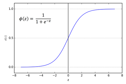
The dot product XW can produce any set of values. However, in our output, we have the values in the form of 1 and 0. We want our output to be in the same format. To do so we need an Activation Function, which restricts the input values between 0 and 1. So of course we’ll go ahead with Sigmoid activation function.

 

The sigmoid function returns 0.5 when the input is 0. It returns a value close to 1 if the input is a large positive number. In the case of negative input, the sigmoid function outputs a value close to zero.

Therefore, it is especially used for models where we have to predict the probability as an output. Since probability of anything exists only between the range of 0 and 1, sigmoid is the right choice for our problem.

In the above figure z is the summation of dot product X.W

Mathematically, the sigmoid activation function is:

 

Let us summarize what we have done so far. First, we have to find the dot product of the input features(matrix of independent variables) with the weights. Next, pass the summation of dot products through an activation function. The result of the activation function is basically the predicted output for the input features.

 

Back Propagation

 
In the beginning, before you do any training, the neural network makes random predictions which are of course incorrect.
We start by letting the network make random output predictions. We then compare the predicted output of the neural network with the actual output. Next, we update the weights and the bias in such a manner that our predicted output comes closer to the actual output. In this phase, we train our algorithm. Let’s take a look at the steps involved in the backpropagation phase.

Step 1: Calculate the cost

The first step in this phase is to find the cost of the predictions. The cost of the prediction can be calculated by finding the difference between the predicted output values and the actual output values. If the difference is large then cost will also be large.

We will use the mean squared error or MSE cost function. A cost function is a function that finds the cost of the given output predictions.

 

Here, Yi is the actual output value and Ŷi is the predicted output value and n is the number of Observations.

Step 2: Minimize the cost

Our ultimate goal is to fine-tune the weights of our neural network in such a way that the cost is minimized the minimum. If you notice carefully, you’ll get to know that we can only control the weights and the bias. Everything else is beyond our control. We cannot control the inputs, we cannot control the dot products, and we cannot manipulate the sigmoid function.

In order to minimize the cost, we need to find the weight and bias values for which the cost function returns the smallest value possible. The smaller the cost, the more correct our predictions are.

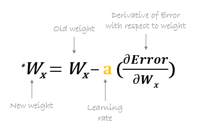
To find the minima of a function, we can use the gradient descent algorithm. The gradient descent can be mathematically represented as:

 

𝛛Error is the cost function. The above equation tells us to find the partial derivative of the cost function with respect to each weight and bias and subtract the result from the existing weights to get new weights.

The derivative of a function gives us its slope at any given point. To find if the cost increases or decreases, given the weight value, we can find the derivative of the function at that particular weight value. If the cost increases with the increase in weight, the derivative will return a positive value which will then be subtracted from the existing value.

On the other hand, if the cost is decreasing with an increase in weight, a negative value will be returned, which will be added to the existing weight value since negative into negative is positive.

In the above equation a is called the learning rate, which is multiplied by the derivative. The learning rate decides how fast our algorithm learns.

We need to repeat the execution of gradient descent for all the weights and biases until the cost is minimized and for which the cost function returns a value close to zero.

Now is the time to implement what we have studied so far. We will create a simple neural network with one input and one output layer in Python.

 

Artificial Neural Network Implementation using numpy

 

 

Steps to follow:
1. Define independent variables and dependent variable
2. Define Hyperparameters
3. Define Activation Function and its derivative
4. Train the model
5. Make predictions

Step-1: Let’s first create our independent variables or input feature set and the corresponding dependent variable or labels.

#Independent variables
input_set = np.array([[0,1,0],
                      [0,0,1],
                      [1,0,0],
                      [1,1,0],
                      [1,1,1],
                      [0,1,1],
                      [0,1,0]])#Dependent variable
labels = np.array([[1,
                    0,
                    0,
                    1,
                    1,
                    0,
                    1]])
labels = labels.reshape(7,1) #to convert labels to vector

Our input set contains seven records. Similarly, we also created a labels set that contains corresponding labels for each record in the input set. The labels are the values that we want our ANN to predict.

Step-2: Define Hyperparameters

we will use the random.seed function of numpy so that we can get the same random values whenever we execute the below code.

Next, we initialize our weights with normally distributed random numbers. Since we have three features in the input, we have a vector of three weights. We then initialize the bias value with another random number. Finally, we set the learning rate to 0.05.

np.random.seed(42)
weights = np.random.rand(3,1)
bias = np.random.rand(1)
lr = 0.05 #learning rate

Step-3: Define Activation Function and it’s derivative: Our activation function is the sigmoid function.

def sigmoid(x):
    return 1/(1+np.exp(-x))

Now define a function that calculates the derivative of the sigmoid function.

def sigmoid_derivative(x):
    return sigmoid(x)*(1-sigmoid(x))

Step-4: Its time to train our ANN model

We’ll start off by defining the number of epochs. An epoch is the number of times we want to train the algorithm on our dataset. We will train the algorithm on our data 25,000 times so our epoch will be 25000. You can try a different number to further decrease the cost.

for epoch in range(25000):
    inputs = input_set
    XW = np.dot(inputs, weights)+ bias
    z = sigmoid(XW)
    error = z - labels
    print(error.sum())
    dcost = error
    dpred = sigmoid_derivative(z)
    z_del = dcost * dpred
    inputs = input_set.T
    weights = weights - lr*np.dot(inputs, z_del)
    
    for num in z_del:
        bias = bias - lr*num

Let’s understand each step one by one and then we will go to our last step of making predictions.

we store the values from the input input_set to the inputs variable so that the value of input_set remain as it is in each iteration and whatever changes are done that must be done to inputs variable.

inputs = input_set

Next, we find the dot product of the input and the weight and add bias to it. (Step-1 of Feedforward phase)

XW = np.dot(inputs, weights)+ bias

Next, We pass the dot product through the sigmoid activation function. (Step-2 of Feedforward phase)

z = sigmoid(XW)

This completes the feedforward part of our algorithm and now is the time to start backpropagation.

The variable z contains the predicted outputs. The first step of the backpropagation is to find the error.

error = z - labels
print(error.sum())

We know that our cost function is:

We need to differentiate this function with respect to each weight and this can be done easily using chain rule of differentiation. I’ll skip the derivation part but if anyone is interested let me know I’ll post it in the comment section.

So our final derivative of the cost function with respect to any weight is:

slope = input x dcost x dpred

Now the slope can be simplified as:

dcost = error
dpred = sigmoid_derivative(z)
z_del = dcost * dpred
inputs = input_set.T
weights = weight-lr*np.dot(inputs, z_del)

we have the z_del variable, which contains the product of dcost and dpred. Instead of looping through each record and multiplying the input with the corresponding z_del, we take the transpose of the input feature matrix and multiply it with the z_del.

Finally, we multiply the learning rate variable lr with the derivative to increase the speed of learning.

Along with updating the weights we also have to update the bias term.

for num in z_del:
        bias = bias - lr*num

Once the loop starts, you will see that the total error starts decreasing and by the end of the training the error is left with a very small value.

-0.001415035616137969
-0.0014150128584959256
-0.0014149901015685952
-0.0014149673453557714
-0.0014149445898578358
-0.00141492183507419
-0.0014148990810050437
-0.0014148763276499686
-0.0014148535750089977
-0.0014148308230825385
-0.0014148080718707524
-0.0014147853213728624
-0.0014147625715897338
-0.0014147398225201734
-0.0014147170741648386
-0.001414694326523502
-0.001414671579597255
-0.0014146488333842064
-0.0014146260878853782
-0.0014146033431002465
-0.001414580599029179
-0.0014145578556723406
-0.0014145351130293877
-0.0014145123710998
-0.0014144896298846701
-0.0014144668893831067
-0.001414444149595611
-0.0014144214105213174
-0.0014143986721605849
-0.0014143759345140276
-0.0014143531975805163
-0.001414330461361444
-0.0014143077258557749
-0.0014142849910631708
-0.00141426225698401
-0.0014142395236186895
-0.0014142167909661323
-0.001414194059027955
-0.001414171327803089
-0.001414148597290995
-0.0014141258674925626
-0.0014141031384067547
-0.0014140804100348098
-0.0014140576823759854
-0.0014140349554301636
-0.0014140122291978665
-0.001413989503678362
-0.001413966778871751
-0.001413944054778446
-0.0014139213313983257
-0.0014138986087308195
-0.0014138758867765552
-0.0014138531655347973
-0.001413830445006264
-0.0014138077251906606
-0.001413785006087985
-0.0014137622876977014
-0.0014137395700206355
-0.0014137168530558228
-0.0014136941368045382
-0.0014136714212651114
-0.0014136487064390219
-0.0014136259923249635
-0.001413603278923519
-0.0014135805662344007
-0.0014135578542581566
-0.0014135351429944293
-0.0014135124324428719
-0.0014134897226037203
-0.0014134670134771238
-0.0014134443050626295
-0.0014134215973605428
-0.0014133988903706311

Step-5: Make predictions

Its time to make some predictions. Let’s try with [1,0,0]

single_pt = np.array([1,0,0])
result = sigmoid(np.dot(single_pt, weights) + bias)
print(result)

Output : [0.01031463]

As you can see the output is closer to 0 than 1 so it is classified as 0.

Let’s try again with [0,1,0]

single_pt = np.array([0,1,0])
result = sigmoid(np.dot(single_pt, weights) + bias)
print(result)

Output : [0.99440207]

As you can see the output is closer to 1 than 0 so it is classified as 1.

 

Conclusion

 
In this article, we learned how to create a very simple artificial neural network with one input layer and one output layer from scratch using numpy python library. This ANN is able to classify linearly separable data.

What if we have non-linearly separated data, our ANN will not be able to classify that type of data. This is what we are going to build in part-2 of this article series.

Well, that’s all. I hope you guys have enjoyed reading this article. Please share your thoughts/doubts in the comment section.

You can reach me out over LinkedIn for any query.

 

Thanks for reading!!!

 
Bio: Nagesh Singh Chauhan is a Big data developer at CirrusLabs. He has over 4 years of working experience in various sectors like Telecom, Analytics, Sales, Data Science having specialisation in various Big data components.

Original. Reposted with permission.

Related: