Backpropagation Algorithm in Neural Network: Examples - Data Analytics

In this post, you will learn about the concepts of neural network backpropagation algorithm along with Python examples. As a data scientist, it is very important to learn the concepts of backpropagation algorithm if you want to get good at deep learning models. This is because back propagation algorithm is key to learning weights at different layers in the deep neural network.

Linear Regression for Machine Learn…

Please enable JavaScript

Linear Regression for Machine Learning | In Detail and Code

What’s Backpropagation Algorithm?

The backpropagation algorithm is a well-known procedure for training neural networks. In general, backpropagation works by propagating error signals backwards through the network, from the output layer back to the input layer. This process adjusts the weights of the connections between neurons in order to minimize the overall error. The backpropagation algorithm represents the propagation of the gradients of outputs from each node (in each layer) on the final output, in the backward direction right up to the input layer nodes. All that is achieved using the backpropagation algorithm is to compute the gradients of weights and biases. Remember that the training of neural networks is done using optimizers and NOT backpropagation. The primary goal of learning in the neural network is to determine how would the weights and biases in every layer would change to minimize the objective or cost function for each record in the training data set. Instead of determining the final output as a function of weights and biases of every layer and take the partial derivatives with respect to weights and biases to determine the gradients, backpropagation makes it simpler to propagate the gradients in the backward direction and help determine the gradients of weights and biases in every layer using the chain rule.

The backpropagation algorithm can be summarized in a few simple steps:

First, the predicted output of the neural network is compared to the actual desired output. This produces an error signal.
Next, this error signal is propagated backwards through the network. That is, it is multiplied by the weights of the connections between neurons and passed back to the previous layer.
The neuron weights and biases are then updated according to this error signal. In general, weights are increased if they contribute to reducing the error, and decreased if they contribute to increasing the error.
This process is then repeated for each layer of the neural network until the error is minimized.

The main idea behind calculating gradients in case of neural network with respect to cost function C is the following:

How do we change weights and biases in every layer (increases or decreases) such that neural network provides output that minimises the cost function?

This is where back propagation algorithm helps in determining direction in which each of the weights and biases need to change to minimise the cost function.

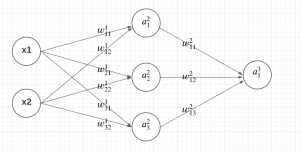
Let’s understand the back propagation algorithm using the following simplistic neural network with one input layer, one hidden layer and one output layer. Let’s take activation function as an identity function for the sake of understanding. In real world problems, the activation functions most commonly used are sigmoid function, ReLU or variants of ReLU functions and tanh function.

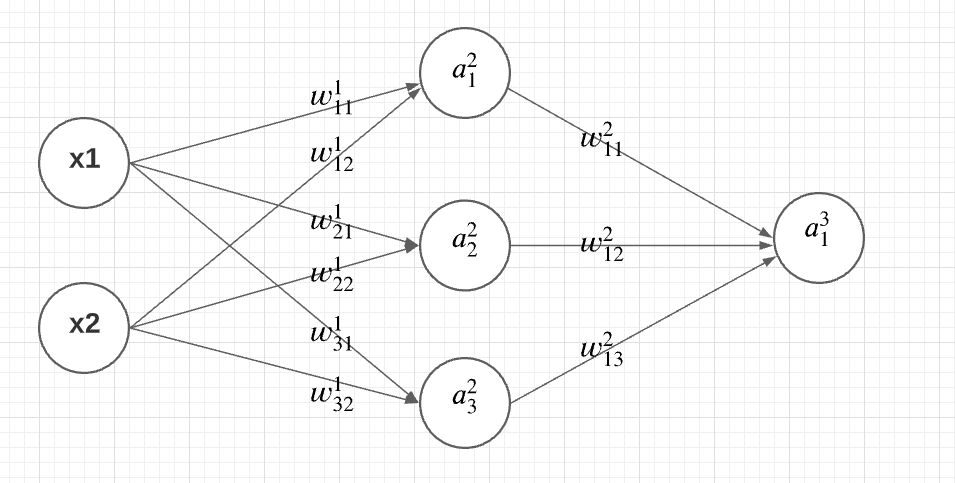Fig 1. Neural Network for understanding Back Propagation Algorithm

Lets understand the above neural network.

There are three layers in the network – input, hidden, and output layer
There are two input variables (features) in the input layer, three nodes in the hidden layer, and one node in the output layer
The activation function of the network is applied to the weighted sum of inputs at each node to calculate the activation value.
The output from nodes in the hidden and output layer is derived from applying the activation function on the weighted sum of inputs to each of the nodes in these layers.

Mathematically, above neural network can be represented as following:

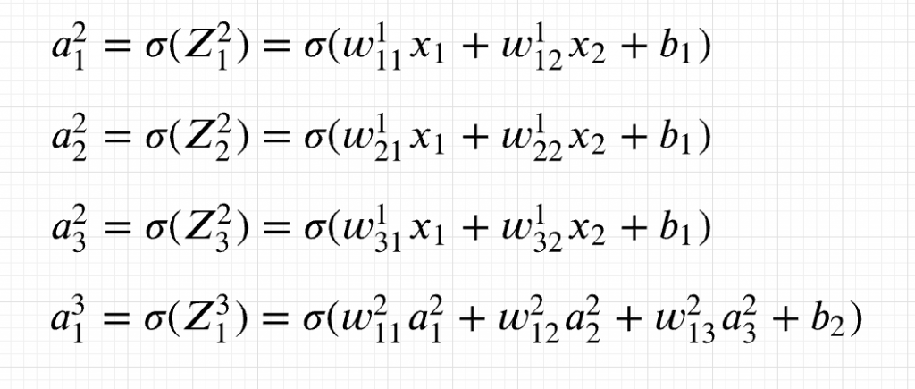Activation function output at different nodes in hidden and output layer

For training the neural network using the dataset, the ask is to determine the optimal value of all the weights and biases denoted by w and b. And, the manner in which the optimal values are found is to optimize / minimize a loss function using the most optimal values of weights and biases. For regression problems, the most common loss function used is ordinary least square function (squared difference between observed value and network output value). For classification problems, the most common loss function used is cross-entropy loss function. For optimizing / minimizing the loss function, the gradient descent algorithm is applied on the loss function with respect to every weights and biases based on back propagation algorithm. The idea is to change or update the weights and biases for every layer in the manner that the loss function reduces after every iteration.

Back propagation algorithm helps in determining gradients of weights and biases with respect to final output value of the network. Once gradients are found, the weights and biases are updated based on different gradient techniques such as stochastic gradient descent. In stochastic gradient descent technique, weights are biases are updated after processing small batches of training data. It is also called as mini-batch gradient descent technique.

The training of neural network shown in the above diagram would mean learning the most optimal value of the following weights and biases in two different layers:

\(\Large w^1_{11}, w^1_{12}, w^1_{21}, w^1_{22}, w^1_{31}, w^1_{32}, b_1\) for the first layer
\(\Large w^2_{11}, w^2_{12}, w^2_{13}, b_2\) for the second layer.

The optimal values for the above mentioned weights and biases in different layers are learned based on their gradients (partial derivatives) and optimization technique such as stochastic gradient descent. The gradients of all the weights and biases with respect to final output is found based on the back propagation algorithm. Here is the list of gradients which is required to be determined with respect to the final output value for learning purpose. If the final output is C (representing cost function), then the gradients can be determined as the following:

\(\Large \frac{\partial C}{\partial w^1_{11}}, \frac{\partial C}{\partial w^1_{12}}, \frac{\partial C}{\partial w^1_{21}}, \frac{\partial C}{\partial w^1_{22}}, \frac{\partial C}{\partial w^1_{31}}, \frac{\partial C}{\partial w^1_{32}}, \frac{\partial C}{\partial b_{1}} \)

\(\Large \frac{\partial C}{\partial w^2_{11}}, \frac{\partial C}{\partial w^2_{12}}, \frac{\partial C}{\partial w^2_{13}}, \frac{\partial C}{\partial b_{2}}\)

Let’s see how back propagation algorithm can be used to determine all of the gradients.

\(\Large \frac{\partial C}{\partial w^2_{11}} = \frac{\partial C}{\partial a^3_1}\frac{\partial a^3_1}{\partial Z^3_1}\frac{\partial Z^3_1}{\partial w^2_{11}} \)

\(\Large \frac{\partial C}{\partial w^2_{12}} = \frac{\partial C}{\partial a^3_1}\frac{\partial a^3_1}{\partial Z^3_1}\frac{\partial Z^3_1}{\partial w^2_{12}} \)

\(\Large \frac{\partial C}{\partial w^2_{13}} = \frac{\partial C}{\partial a^3_1}\frac{\partial a^3_1}{\partial Z^3_1}\frac{\partial Z^3_1}{\partial w^2_{13}} \)

\(\Large \frac{\partial C}{\partial w^1_{11}} = \frac{\partial C}{\partial a^3_1}\frac{\partial a^3_1}{\partial Z^3_1}\frac{\partial Z^3_1}{\partial a^2_1}\frac{\partial a^2_1}{\partial Z^2_1}\frac{\partial Z^2_1}{\partial w^1_{11}}\)

\(\Large \frac{\partial C}{\partial w^1_{12}} = \frac{\partial C}{\partial a^3_1}\frac{\partial a^3_1}{\partial Z^3_1}\frac{\partial Z^3_1}{\partial a^2_1}\frac{\partial a^2_1}{\partial Z^2_1}\frac{\partial Z^2_1}{\partial w^1_{12}}\)

\(\Large \frac{\partial C}{\partial w^1_{21}} = \frac{\partial C}{\partial a^3_1}\frac{\partial a^3_1}{\partial Z^3_2}\frac{\partial Z^3_2}{\partial a^2_2}\frac{\partial a^2_2}{\partial Z^2_2}\frac{\partial Z^2_2}{\partial w^1_{21}}\)

\(\Large \frac{\partial C}{\partial w^1_{22}} = \frac{\partial C}{\partial a^3_1}\frac{\partial a^3_1}{\partial Z^3_2}\frac{\partial Z^3_2}{\partial a^2_2}\frac{\partial a^2_2}{\partial Z^2_2}\frac{\partial Z^2_2}{\partial w^1_{22}}\)

\(\Large \frac{\partial C}{\partial w^1_{31}} = \frac{\partial C}{\partial a^3_1}\frac{\partial a^3_1}{\partial Z^3_1}\frac{\partial Z^3_1}{\partial a^2_3}\frac{\partial a^2_3}{\partial Z^2_3}\frac{\partial Z^2_3}{\partial w^1_{31}}\)

\(\Large \frac{\partial C}{\partial w^1_{32}} = \frac{\partial C}{\partial a^3_1}\frac{\partial a^3_1}{\partial Z^3_1}\frac{\partial Z^3_1}{\partial a^2_3}\frac{\partial a^2_3}{\partial Z^2_3}\frac{\partial Z^2_3}{\partial w^1_{32}}\)

The above equations represents the aspect of how cost function C value will change by changing the respective weights in different layers. In other words, the above equations calculates gradients of weights and biases with respect to cost function value, C. Note how chain rule is applied while calculating gradients using back propagation algorithm.

You may want to check this post to get an access to some real good articles and videos on back propagation algorithm – Top Tutorials – Neural Network Back Propagation Algorithm.

Learning Weights & Biases using Back Propagation Algorithm

The equation below represents how weights & biases in specific layers are updated after the gradients are determined. Letter l is used to represent the weights of different layers

\(\large w^l = w^l – learningRate * \frac{\partial C}{\partial w^l}\)

\(\large b^l = b^l – learningRate * \frac{\partial C}{\partial b^l}\)

Conclusions

That’s all for this overview of the backpropagation algorithm used in the neural network. If you would like to know more, or have any questions, please let me know in the comments below and I will do my best to answer them. Have a great day!