
Activation Functions in Deep Learning: Sigmoid, tanh, ReLU – KI Tutorials
In this guide, I will introduce you to four of the most important activation functions used in Deep Learning: Sigmoid, Tanh, ReLU & Leaky ReLU. Specifically, this guide will cover what activation functions are when we need to use which activation functions, and how to implement them in practice in TensorFlow.
Short answer: We need to use activation functions such as ReLu, sigmoid, and tanh to give the neural network a non-linear property. This way, the network can model more complex relationships and patterns in the data.
Mục Lục
Content Overview
- What is an activation function?
- Recap: Forward Propagation
- Neural network is a function
- Why do we need activation functions?
- Different types of activation functions (sigmoid, tanh, ReLU, leaky ReLU, softmax).
- Which activation functions should we use?
1. What is an Activation Function?
An activation function determines the range of values of activation of an artificial neuron. This is applied to the sum of the weighted input data of the neuron. An activation function is characterized by the property of non-linearity. Without the application of an activation function, the only operations in computing the output of a multilayer perceptron would be the linear products between the weights and the input values.
Linear operations performed in succession can be considered as a single linear operation. On the other hand, the application of the non-linear activation function leads to a non-linearity of the artificial neural network and thus to a non-linearity of the function that approximates the neural network. According to the approximation theorem, a multilayer perceptron with only one hidden layer using a nonlinear activation function is a universal function approximator.
Four of the most common activation functions used in practice are presented below.
2. Recapitulation: Forward Propagation
To understand the meaning of activation functions, we must first discuss how a neural network computes a prediction/output. This is generally referred to as forward propagation. In forward propagation, the neural network receives an input vector  and computes a prediction vector
  . How does something like this work?
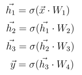
Please consider the following neural network with one input, one output, and three hidden layers:
Fig. 1 Schematic representation of a neural network
Each layer of the network is connected to the next layer by a so-called weight matrix. In total, we have four weight matrices  ,
,  ,
,  , and
, and  in the example in Fig. 1.
Given an input vector , we calculate a product with the first weight matrix and apply the activation function to the result of this product. The result is a new vector  representing the values of the neurons in the first layer. This vector is used as the new input vector for the next layer, where the same operations are performed again. This is repeated until we get the final output vector , which is considered as the prediction of the neural network.
The entire set of operations can be represented by the following equations, where σ is an arbitrary activation function:
 Equation 1. Calculation of output in a neural network.
3. Neural Network is a Function
At this point, I would like to discuss with you another interpretation that can be used to describe a neural network. Instead of thinking of a neural network as a collection of neurons and connections, we can think of the neural network simply as a function.
Like any ordinary mathematical function, a neural network performs a mathematical mapping from input  to output
  .
.
The concept of computing an output for an input is probably already familiar to you. It is the concept of an ordinary mathematical function. In mathematics, we can define a function  as follows:
Equation 2. Example of a basic mathematical function.
This function takes three inputs  ,
,  , and
, and  .
.  ,
,  ,
,  are the function parameters that take specific values. Given the inputs , , and , the function computes an output .
Basically, this is exactly how a neural network works. We take an input vector and input it into the neural network. The neural network, in turn, computes an output using the input .
So instead of thinking of a neural network as a simple collection of neurons and connections, we can think of a neural network as a function. This function includes all the computations that we previously considered separately in Equation 1 as a single, concatenated computation:
Equation 3. A neural network as a function.
In Equation 2, the simple mathematical function we considered had parameters , , and determining the output value of for an input .
In the case of a neural network, the parameters of the corresponding function are the weights. This means that our goal in training a neural network is to find a particular set of weights or parameters so that, given an input vector , we can compute a prediction that corresponds to the actual target value (label)  .
.
In other words: We are trying to create a function that can model our training data.
One question you may be asking is: can we always model arbitrary data with a neural network? Can we always find weights that define a function that can compute a given prediction y for given features x? The answer is no. We can only model the data if there exists a mathematical dependency between the input vector and the labels .
This mathematical dependence can vary in complexity. And in most cases, we as humans cannot see this relationship with our eyes when we take a look at the data. However, if there is a mathematical dependency between the input vectors and the labels, we can be sure that the neural network will recognize this dependency during training and adjust the weights so that it can model this dependency in the training data. Or, in other words, so that it can realize a mathematical mapping from input features to output .
4. Why do we need Activation Functions?
The purpose of an activation function is to provide some sort of non-linear property to the neural network. Without the activation functions, the neural network could only compute linear mappings from inputs to outputs . Why is this so?
Without the activation functions, the only mathematical operation during the forward propagation would consist of products between an input vector and a weight matrix.
Since a single product is a linear operation, multiple consecutive products would be nothing more than multiple linear operations repeated in sequence. And multiple, successive linear operations can be considered as a single linear operation.
In order to compute really interesting things, neural networks need to be able to approximate non-linear relationships between input vectors and outputs . The more complex the data we are trying to learn something from, the more “non-linear” the mapping from to tends to be.
A neural network that does not have an activation function in the hidden layer would not be able to mathematically realize such complex relationships, and would not be able to solve the tasks we are trying to solve with the network.
5. The four most important Activation Functions in Deep Learning
At this point, we should discuss the main activation functions used in Deep Learning and their advantages and disadvantages.
4.1 Sigmoid Function
A few years ago, probably the most common activation function was the sigmoid function. The sigmoid function maps the incoming inputs to a range between 0 and 1:
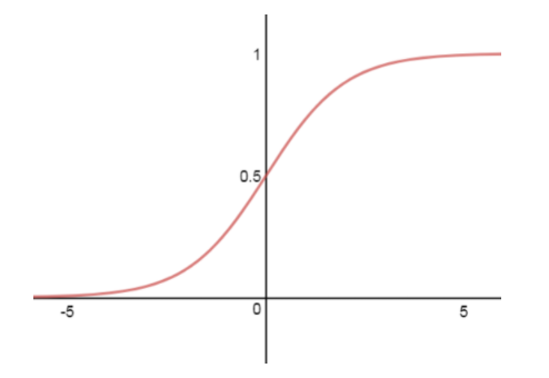 Fig. 2 Sigmoid function.
The mathematical definition of the sigmoid function is as follows:
 Equation 4 Math. Definition of the sigmoid function.
The function takes an input value and returns the output in the interval (0, 1]). In practice, the sigmoid nonlinearity has recently fallen out of favor and is rarely used. It has two main drawbacks:
Sigmoid “kills” gradients
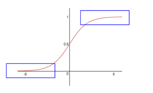
The first is that gradients can disappear in sigmoid functions. A very undesirable property of the function is that the activation of neurons saturates either near 0 or near1 (blue areas):
 Sigmoid function.
The derivative of the sigmoid function becomes very small for these blue areas (i.e., large negative or positive input values). In this case, the derivative near zero would make the gradient of the loss function very small, preventing the updating of the weights and thus the entire learning process.
Sigmoid is not zero-centered
Another undesirable property of sigmoid activation is that the outputs of the function are not zero-centered. This usually makes training the neural network more difficult and unstable.
Consider a “sigmoid” neuron with inputs and , weighted by  and
and  :
:
![]()
and are the outputs of a previous hidden layer with sigmoidal activation. Thus, and are always positive because the sigmoid is not zero-centered. Depending on the gradient of the entire expression  , the gradient with respect to and is always either positive for and or negative for and .
Often the optimal gradient descent step requires an increase in and a decrease in . Thus, since and are always positive, we cannot increase and decrease the weights simultaneously; we can only increase or decrease all the weights simultaneously.
We can implement the sigmoid function in TensorFlow with the following code:
import tensorflow as tf
from tensorflow.keras.activations import sigmoid

z = tf.constant([-1.5, -0.2, 0, 0.5], dtype=tf.float32)
output = sigmoid(z)

print(output.numpy()) #[0.18242553, 0.45016602, 0.5, 0.62245935]
4.2 Tanh Activation Function
Another activation function very commonly used in Deep Learning is the Tanh function. The tangent hyperbolic function is shown in the following figure:
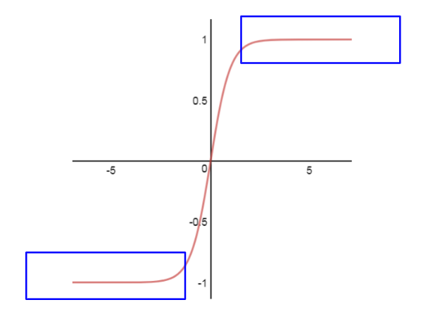 Fig. 3 Tanh function
The function maps a real-valued number to the range [-1, 1] according to the following equation:
 Equation. 5 Math. Definition of the Tanh function.
As with the sigmoid function, neurons saturate at large negative and positive values, and the derivative of the function approaches zero (blue region in Fig. 3). However, unlike the sigmoid function, its outputs are zero-centered. Therefore, in practice, the tanh function is always preferred to the sigmoid function.
We can implement the tanh function in TensorFlow with the following code:
import tensorflow as tf
from tensorflow.keras.activations import tanh

z = tf.constant([-1.5, -0.2, 0, 0.5], dtype=tf.float32)
output = tanh(z)

print(output.numpy()) # [-0.90514827, -0.19737533,  0., 0.46211714]
4.3 Rectified Linear Unit – ReLU
The Rectified Linear Unit or simply ReLU has become very popular in recent years. The activation is linear for input values greater than zero:  or more precisely:
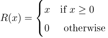 Equation 6. Math. definition of the ReLU function
For inputs greater than zero, we obtain a linear mapping:
 Fig. 4 ReLU
There are several advantages and disadvantages of using ReLUs:
- (+) In practice, ReLU has been shown to accelerate the convergence of the gradient descent toward the global minimum of the loss function compared to other activation functions. This is due to its linear, non-saturating property.
- (+) While other activation functions (tanh and sigmoid) require very computationally expensive operations such as exponents, etc., ReLU, on the other hand, can be implemented simply by thresholding a value vector at zero.
- (-) Unfortunately, there is also a problem with the ReLU activation function. Since the outputs of this function are zero for input values below zero, the neurons of the network can become very fragile and even “die” during training. What is meant by this? It may (need not, but can) happen that when the weights are updated, the weights are adjusted in a way that for certain neurons of a hidden layer the inputs
 are always below zero. This means that the values f(x) of these neurons (with f as the ReLU function) are always zero (
 ) and thus make no contribution to the training process. This means that the gradient flowing through these ReLU neurons is also zero from that point on. We say that the neurons are “dead.” For example, it is very common to observe that 20-50% of the entire neural network that used the ReLU function is “dead”. In other words, these neurons are never activated in the entire dataset used in training.
We can implement the ReLU function in TensorFlow with the following code:
import tensorflow as tf
from tensorflow.keras.activations import relu

z = tf.constant([-1.5, -0.2, 0, 0.5], dtype=tf.float32)
output = relu(z)
print(output.numpy()) #[0.  0.  0.  0.5]
4.4 Leaky ReLU
Leaky ReLu is nothing more than an improved version of the ReLU activation function. As mentioned in the previous section, using ReLU may “kill” some neurons in our neural network and these neurons may never become active again.
Leaky ReLU was defined to solve this problem. Unlike “vanilla” ReLU, where all values of the neurons are zero for input values , in the case of Leaky ReLU we add a small linear component to the function:
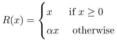 Fig. 5 Math. definition of Leaky-ReLU
Leaky-ReLU activation looks as follows:
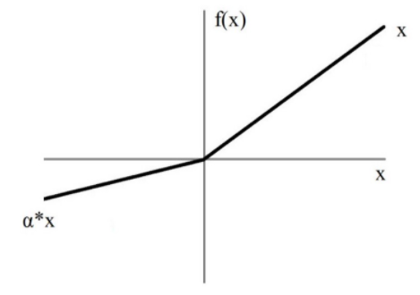 Fig. 6 Leaky ReLU.
Basically, we have replaced the horizontal line for values below zero with a non-horizontal linear line. The slope of this linear line can be set by the parameter  , which is multiplied by the input .
The advantage of using Leaky ReLU and replacing the horizontal line is that we avoid zero gradients. This is because in this case we no longer have “dead” neurons that are always zero and thus no longer contribute to the training.
We can implement the leaky RLU function in TensorFlow with the following code:
import tensorflow as tf
from tensorflow.keras.layers import LeakyReLU

leaky_relu = LeakyReLU(alpha=0.01)
z = tf.constant([-1.5, -0.2, 0, 0.5], dtype=tf.float32)
output=leaky_relu(z)

print(output.numpy()) # [-0.015, -0.002,  0.,0.5]
4.5 Softmax Activation Function
Last but not least, I would like to introduce the softmax activation function. This activation function is quite unique.
Softmax is only applied in the last layer and only when the neural network is asked to predict probability values in classification tasks.
Simply put, the softmax activation function forces the values of the output neurons to take values between zero and one, so that they can represent probability values in the interval [0, 1].
Another point to consider is that when input features are classified into different classes, these classes are mutually exclusive. This means that each feature vector belongs to only one class. This means that a feature vector that is an image of a dog cannot represent the class dog with a probability of 50% and the class cat with a probability of 50%. This feature vector must represent the dog class with a probability of 100%.
Furthermore, for mutually exclusive classes, the probability values of all output neurons must sum to one. Only in this way does the neural network represent a correct probability distribution. A counterexample would be a neural network that classifies the image of a dog into the class dog with a probability of 80% and into the class cat with a probability of 60%.
Fortunately, the softmax function not only forces the outputs into the range between 0 and 1, but also ensures that the sum of the outputs across all possible classes adds up to one. Let’s now take a look at how the softmax function works.
Fig. 7 Softmax activation in the last layer of the network.
Imagine that the neurons in the output layer receive an input vector  , which is the result of a product between a weight matrix of the current layer and the output of the previous layer. A neuron in the output layer with softmax activation receives a single value
  , which is an entry in the vector , and outputs the value
  .
.
When we use softmax activation, each single output of a neuron in the output layer is calculated according to the following equation:
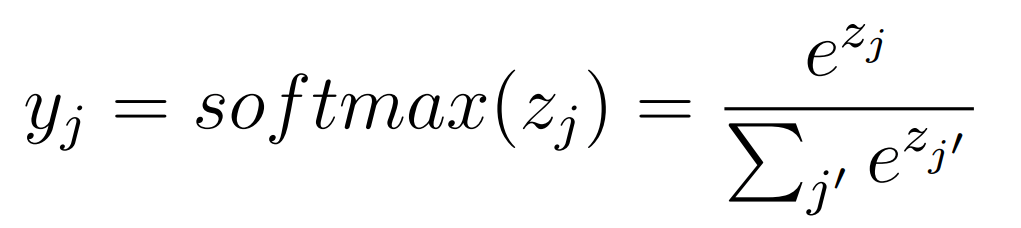 Eq. 7 Math. definition of the softmax function.
As you can see, each value  of a particular neuron depends not only on the value
  that the neuron receives, but on all the values in the vector . This makes each value of an output neuron a probability value between 0 and 1. And the probability predictions over all output neurons sum to one.
In this way, the output neurons now represent a probability distribution over the mutually exclusive class labels.
5. Which Activation Functions should we use?
I will answer this question with the best answer there is: It depends. ¯\_(ツ)_/
In particular, it depends on the problem you are trying to solve and the range of values of the output you expect.
For example, if you want your neural network to predict values greater than 1, then tanh or sigmoid are not appropriate for the output layer, and we must use ReLU instead.
On the other hand, if we expect the output values to be in the range [0,1] or [-1, 1], then ReLU is not a good choice for the output layer and we must use sigmoid or tanh.
If you are performing a classification task and want the neural network to predict a probability distribution over the mutually exclusive class labels, then the softmax activation function should be used in the last layer.
However, as far as hidden layers are concerned, as a rule of thumb, I would recommend always using ReLU as the activation for these layers.
Take-Home-Message
- Activation functions add a nonlinear property to the neural network. This allows the network to model more complex data.
- ReLU should generally be used as an activation function in the hidden layers.
- In the output layer, the expected value range of the predictions must always be considered.
- For classification tasks, I recommend using only softmax activation in the output layer
©KI Tutorials


![Toni Kroos là ai? [ sự thật về tiểu sử đầy đủ Toni Kroos ]](https://evbn.org/wp-content/uploads/New-Project-6635-1671934592.jpg)


