Activation Functions: Sigmoid vs Tanh | Baeldung on Computer Science

Mục Lục

1. Overview

In this tutorial, we’ll talk about the sigmoid and the tanh activation functions. First, we’ll make a brief introduction to activation functions, and then we’ll present these two important functions, compare them and provide a detailed example.

2. Activation Functions

An essential building block of a neural network is the activation function that decides whether a neuron will be activated or not. Specifically, the value of a neuron in a feedforward neural network is calculated as follows:

$Y = \sum_{i=1}^m (x_i * w_i) + b$

where $x_i$ are the input features, $w_i$ are the weights, and $b$ is the bias of the neuron. Then, an activation function $\mathbf{f}$ is applied at the value of every neuron and decides whether the neuron is active or not:

$output = f(Y)$

In the figure below, we can see diagrammatically how an activation function works:

neuron

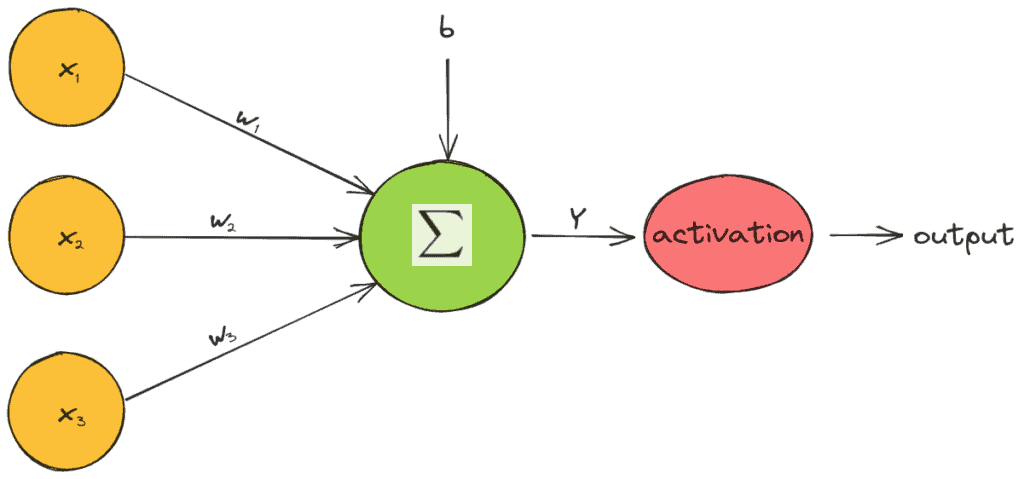
The activation functions are univariate and non-linear since a network with a linear activation function is equivalent to just a linear regression model. Due to the non-linearity of activation functions, neural networks can capture complex semantic structures and achieve high performance.

3. Sigmoid

The sigmoid activation function (also called logistic function) takes any real value as input and outputs a value in the range $\mathbf{(0, 1)}$ . It is calculated as follows:

$\mathbf{s(x) = \frac{1}{1 + e^{-x}}}$

where $x$ is the output value of the neuron. Below, we can see the plot of the sigmoid function when the input lies in the range $[-10, 10]$ :

sigmoid

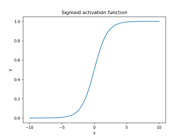
As expected, the sigmoid function is non-linear and bounds the value of a neuron in the small range of $(0, 1)$ . When the output value is close to 1, the neuron is active and enables the flow of information, while a value close to 0 corresponds to an inactive neuron.

Also, an important characteristic of the sigmoid function is the fact that it tends to push the input values to either end of the curve (0 or 1) due to its S-like shape. In the region close to zero, if we slightly change the input value, the respective changes in the output are very large and vice versa. For inputs less than -5, the output of the function is almost zero, while for inputs greater than 5, the output is almost one.

Finally, the output of the sigmoid activation function can be interpreted as a probability since it lies in the range $[0, 1]$ . That’s why it is also used in the output neurons of a prediction task.

4. Tanh

Another activation function that is common in deep learning is the tangent hyperbolic function simply referred to as tanh function. It is calculated as follows:

$\mathbf{tanh(x) = \frac{e^{x} - e^{-x}}{e^{x} + e^{-x}} = \frac{1 - e^{-2x}}{1 + e^{-2x}} = \frac{2 - (1 + e^{-2x})}{1 + e^{-2x}}= \frac{2}{1 + e^{-2x}} - 1 = 2s(2x) - 1}$

We observe that the tanh function is a shifted and stretched version of the sigmoid. Below, we can see its plot when the input is in the range $[-10, 10]$ :

tanh

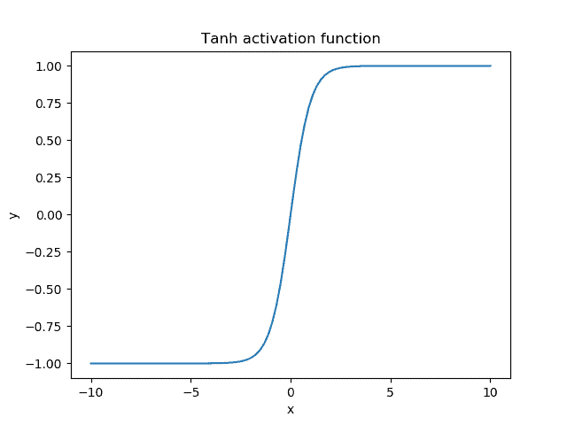
The output range of the tanh function is $(-1, 1)$ and presents a similar behavior with the sigmoid function. The main difference is the fact that the tanh function pushes the input values to 1 and -1 instead of 1 and 0.

5. Comparison

Both activation functions have been extensively used in neural networks since they can learn very complex structures. Now, let’s compare them, presenting their similarities and differences.

5.1. Similarities

As we mentioned earlier, the tanh function is a stretched and shifted version of the sigmoid. Therefore, there are a lot of similarities.

Both functions belong to the S-like functions that suppress the input value to a bounded range. This helps the network to keep its weights bounded and prevents the exploding gradient problem where the value of the gradients becomes very large.

5.2. Differences

An important difference between the two functions is the behavior of their gradient. Let’s compute the gradient of each activation function:

$s'(x) = s(x) (1 - s(x))$

$tanh'(x) = 1 - tanh^2(x)$

Below, we plot the gradient of the sigmoid (red) and the tanh (blue) activation function:

derivatives

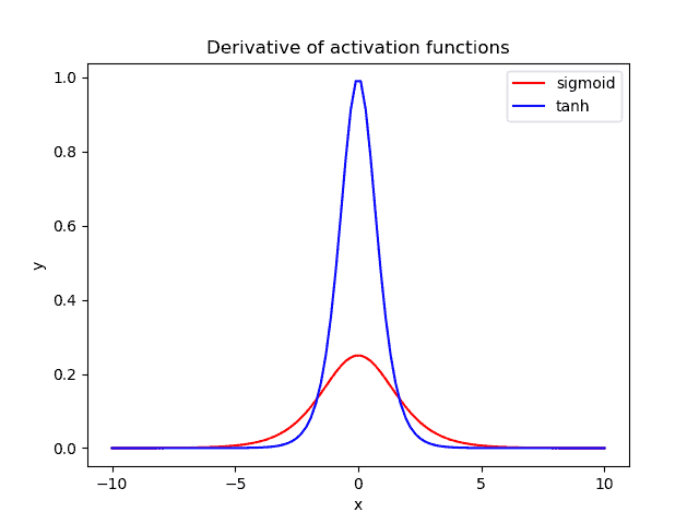
When we are using these activation functions in a neural network, our data are usually centered around zero. So, we should focus our attention on the behavior of each gradient in the region near zero.

We observe that the gradient of tanh is four times greater than the gradient of the sigmoid function. This means that using the tanh activation function results in higher values of gradient during training and higher updates in the weights of the network. So, if we want strong gradients and big learning steps, we should use the tanh activation function.

Another difference is that the output of tanh is symmetric around zero leading to faster convergence.

6. Vanishing Gradient

Despite their benefits, both functions present the so-called vanishing gradient problem.

In neural networks, the error is backpropagated through the hidden layers of the network and updates the weights. In case we have a very deep neural network and bounded activation functions like the ones above, the amount of error decreases dramatically after it is backpropagated through each hidden layer. So, at the early layers, the error is almost zero, and the weights of these layers are not updated properly. The ReLU activation function can fix the vanishing gradient problem.

7. Example

Finally, we’ll present an example of applying these activation functions in a simple neuron of two input features $x_1 = 0.1, x_2 = 0.4$ and weights $w_1 = 0.5, w_2 = -0.5$ . Below, we can see the output value and the gradient when we use the sigmoid (left) and the tanh (right) activation function:

activation example

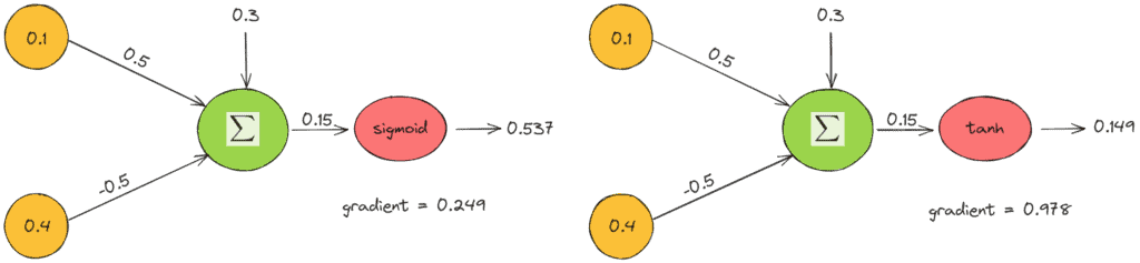
The above example verifies our previous comments. The output value of tanh is closer to zero, and the gradient is four times greater.

8. Conclusion

In this tutorial, we talked about two activation functions, the tanh and the sigmoid. First, we introduced the term, and then we described and compared the two functions along with an example.