What Is a Neural Network? An Introduction with Examples

We want to explore machine learning on a deeper level by discussing neural networks. We will do that by explaining how you can use TensorFlow to recognize handwriting. But to do that we first must understand what are neural networks.

We begin our discussion, based upon our knowledge of linear models, and draw some introductory material from this book written by Michael Nielsen. It is recommended by TensorFlow.

Mục Lục

What are neural networks?

To begin our discussion of how to use TensorFlow to work with neural networks, we first need to discuss what neural networks are.

Think of the linear regression problem we have look at several times here before. We have the concept of a loss function. A neural network hones in on the correct answer to a problem by minimizing the loss function.

Suppose we have this simple linear equation: y = mx + b. This predicts some value of y given values of x.

Predictive models are not always 100% correct. The measure of how incorrect it is is the loss. The goal of machine learning it to take a training set to minimize the loss function. That is true with linear regression, neural networks, and other ML algorithms.

For example, suppose m = 2, x = 3, and b = 2. Then our predicted value of y = 2 * 3 + 2 = 8. But our actual observed value is 10. So the loss is 10 – 8 = 2.

What are perceptrons?

In a neural network, we have the same basic principle, except the inputs are binary and the outputs are binary. The objects that do the calculations are perceptrons. They adjust themselves to minimize the loss function until the model is very accurate. For example, we can get handwriting analysis to be 99% accurate.

Neural networks are designed to work just like the human brain does. In the case of recognizing handwriting or facial recognition, the brain very quickly makes some decisions. For example, in the case of facial recognition, the brain might start with “It is female or male? Is it black or white? Is it old or young? Is there a scar?” and so forth.

Michael Nielsen lays this out in his book like the diagram below. All of these inputs (x1, x2, x3) are fed into a perceptron. That then makes a yes or no decision and passes it onto the next perceptron for the next decision. This process repeats until the final perceptron. At which point we know what the handwriting is or whose face we are looking at.

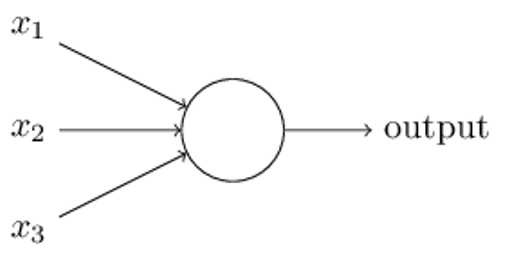
Let’s illustrate with a small example. This topic is complex, so we will present the first concept here and in the next post take it a step further.

As we said, a perceptron is an object that takes binary inputs and outputs a binary output. It uses a weighted sum and a threshold to decide whether the outcome should be yes (1) or no (0).

For example, suppose you want to go to France but only if:

x1 -> The airline ticket is less than $1,000.
x2 -> Your girlfriend or boyfriend can go with you.

You represent this decision with this simple vector of possible inputs:

(1,0), (0,1), (1,1), and (0,0).

In the first case (1,0) the ticket is > 1,000 and your girlfriend or boyfriend cannot go with you.

You put some weight on each of these two calculations. For example, if you are on a budget and cost is important, give it weight w1=4. And whether your partner can go or not is not as important. So give it a weight of w2=3.

So you have this function for Go to France:

(x1 * w1) + (x2 * w2) = (x1 * 4) + (x2 * 3) > some threshold, b, say, 4.

We move b to the other side and write:

If (x1 * 4) + (x2 * 3) -4 > 0 then Go to France (i.e., perceptron says 1)-

Then feed vectors into the equation. Obviously if the ticket is > $1,000 and if your girlfriend cannot go (0,0) then you will not make the trip, because

(0 * 3) + (0 * 4) – 4 is obviously < 0.

If the ticket is cheap but you are going alone then go anyway:

(1 * 4) + (0 * 3) – 4 = 0 which is not bigger than 0.

Handwriting recognition with Neural Networks

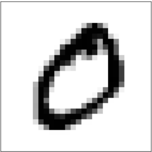
Handwriting and facial recognition using neural networks does the same thing, meaning making a series of binary decisions. This is because any image can be broken down into its smallest object, the pixel. In the case of handwriting, like shown below, each pixel is either black (1) or white (meaning empty, or 0).

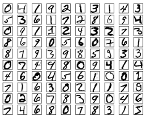
Image Recognition with Neural Networks

Already we introduced the concept of perceptrons, which take inputs from simple linear equations and output 1 (true) or 0 (false). They are the left-hand side of the neural network.

But as Michael Nielsen explains, in his book, perceptrons are not suitable for tasks like image recognition because small changes to the weights and biases product large changes to the output. After all, going to 0 to 1 is a large change. It would be better to go from, say, 0.6 to 0.65.

Suppose have a simple neural network with two input variables x1 and x2 and a bias of 3 with weights of -2 and -3. The equation for that is:

If -2×1 + -3×2 + 3 < 0 then 1 (true) otherwise 0 (false).

(That’s not exactly the correct way to express that in algebra, but it is close enough. The goal here is to keep the math to a minimum to make it easier to understand. Michael’s paper is difficult to understand for those without a math background.)

Machine learning adjusts the weights and the biases until the resulting formula most accurately calculates the correct value. Remember from the last post, that this is the same as saying that adjusting the weights and biases reduces the loss function to its minimum. Most ML problems work that way. For example, linear regression.

So how do we avoid the large change of going from 0 to 1, which would mess up our model? We allow inputs and output numbers between 0 and 1 instead of just 0 or 1.

The simplest way to do that is to divide the equation into the number 1, by using a similar formula, as that used by logistic regression. And then we adopt the convention that if the final output value of the neural network has a threshold, say 0.5, then we can conclude that the outcome is 1.

But isn’t that just a roundabout way of calculating something that results in either 0 or 1? No. Because in a neural network there is not just the input initial values and the resulting output. In the middle, there are intermediate steps called hidden layers. Those need not evaluate to 0 or 1.

(You can play around with a neural network to add or remove hidden layers using this online tool.)

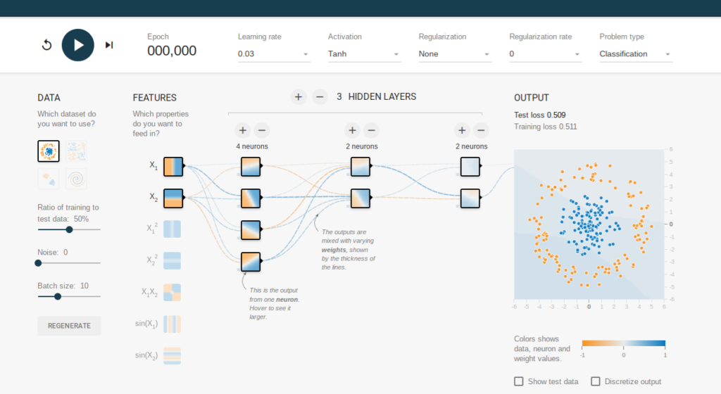
To illustrate, let z=x1w1 + x2w2 + b be the function above. Then we create a modified perception called a sigmoid neuron function (δ) like this.

Now we state that the values of x1 and x2 in function z do not have to be integers. They can be any value between 0 and 1, as a result of which the sigmoid neuron function δ will vary between 0 and 1.

Remember that exp,the constant e = 2.714. Raising it to a negative power is the same as dividing it into 1, i.e. exp(-z) = 1 / exp(z).

When the value of z is large then exp(-z) is small (close to zero). Because 1 divided by something large is small. In that case, the sigmoid neuron function is close to 1. Conversely, when z is small then 1/(1 + exp(-z) is close to 0. But for values that are neither large nor small, δ does not vary much.

Neural Network Training

With artificial intelligence, we train the neural network by varying the weights x1, x2, x3, … , xn and the bias b. That is to say, we vary the inputs to minimize the loss function. That is no different than simple linear regression.

Remember that the loss function is just the difference between the predicted value and the observed value. When there is just 1 or 2 inputs that is easy. But with handwriting recognition there are hundreds or thousands of inputs.

(For an image of 256 pixels there are 256 * 256 inputs in our neural network, it looks something like this, except that this has been made smaller so that you can visualize it. And this network only looks at digits and not the whole alphabet.)

With simple linear regression, the loss function is the distance between the observed value z and the predicted value p, or z – p. With neural networks we use something more complicated called the stochastic gradient descent, which is not necessary to be understood.It will suffice to say that it is basically the same thing. But finding the minimum value in some function with thousands of input variables is hard to achieve, so the stochastic gradient descent first takes a guess and then works from there.

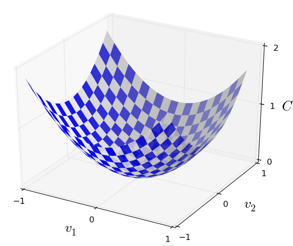
Michael Nielsen gives this analogy. Below is a graph of a loss function f(x,y), i.e. a function with two inputs. If you drop a marble into that bowl then it will roll to the lowest point. The stochastic gradient descent is an algorithm to find that point for a loss function with many input variables. (For those who know calculus, you might say why not just take the derivative of that function and find its minimum? The answer is that you cannot easily find the derivative for a function with thousands of variables.)

Anyway, let’s now see how this works with handwriting recognition. Here is an image of the number “0”. The neural network looks at each pixel, and how dark the pixel is, to figure out which pixels are filled in. Then it matches that with handwriting samples known to represent the number 0.

The MNIST training set takes handwriting samples from 250 people. This data takes the combination of pixels of each drawing and indicates whether it is a 0, 1, 2, …, or 9.

The neural network is then trained, based on this data, i.e., it adjusts the coefficients and bias until it most accurately determines what digit it is.

Then you plug in handwriting samples from people who are not present in the training set. This new set of data is called the testing set, which makes it possible to read what these people have written.